雖然作者曾在

文本中，以『變換』思維視野之重要性，簡略的介紹了

Laplace transform︰

生成函數『形式』何其多？

『變換』思維道其妙︰

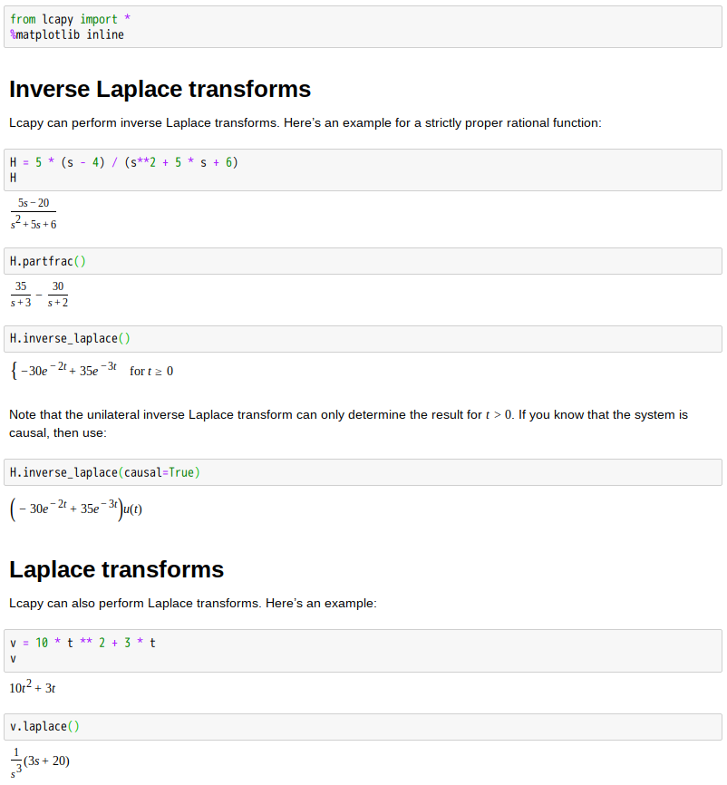
Laplace transform

In mathematics the Laplace transform is an integral transform named after its discoverer Pierre-Simon Laplace (/ləˈplɑːs/). It takes a function of a positive real variable $t$ (often time) to a function of a complex variable $s$ (frequency).

The Laplace transform is very similar to the Fourier transform. While the Fourier transform of a function is a complex function of a real variable (frequency), the Laplace transform of a function is a complex function of a complex variable. Laplace transforms are usually restricted to functions of $t$ with $t > 0$ . A consequence of this restriction is that the Laplace transform of a function is a holomorphic function of the variable $s$ . Unlike the Fourier transform, the Laplace transform of a distribution is generally a well-behaved function. Also techniques of complex variables can be used directly to study Laplace transforms. As a holomorphic function, the Laplace transform has a power series representation. This power series expresses a function as a linear superposition of moments of the function. This perspective has applications in probability theory.

The Laplace transform is invertible on a large class of functions. The inverse Laplace transform takes a function of a complex variable s (often frequency) and yields a function of a real variable t (time). Given a simple mathematical or functional description of an input or output to a system, the Laplace transform provides an alternative functional description that often simplifies the process of analyzing the behavior of the system, or in synthesizing a new system based on a set of specifications.^[1] So, for example, Laplace transformation from the time domain to the frequency domain transforms differential equations into algebraic equations and convolution into multiplication. It has many applications in the sciences and technology.

『對數』概念始其用︰

歐拉公式 $e^{i \theta} = \cos(\theta) + i \sin(\theta)$ 開其門︰

歷代耕耘方法傳。

History

The Laplace transform is named after mathematician and astronomer Pierre-Simon Laplace, who used a similar transform (now called the z-transform) in his work on probability theory.^[2] The current widespread use of the transform (mainly in engineering) came about during and soon after World War II ^[3] although it had been used in the 19th century by Abel, Lerch, Heaviside, and Bromwich.

The early history of methods having some similarity to Laplace transform is as follows. From 1744, Leonhard Euler investigated integrals of the form

z=\int X(x)e^{ax}\,dx\quad {\text{ and }}\quad z=\int X(x)x^{A}\,dx

as solutions of differential equations but did not pursue the matter very far.^[4]

Joseph Louis Lagrange was an admirer of Euler and, in his work on integrating probability density functions, investigated expressions of the form

\int X(x)e^{-ax}a^{x}\,dx,

which some modern historians have interpreted within modern Laplace transform theory.^[5]^[6]^{[clarification needed]}

These types of integrals seem first to have attracted Laplace’s attention in 1782 where he was following in the spirit of Euler in using the integrals themselves as solutions of equations.^[7] However, in 1785, Laplace took the critical step forward when, rather than just looking for a solution in the form of an integral, he started to apply the transforms in the sense that was later to become popular. He used an integral of the form

\int x^{s}\phi (x)\,dx,

akin to a Mellin transform, to transform the whole of a difference equation, in order to look for solutions of the transformed equation. He then went on to apply the Laplace transform in the same way and started to derive some of its properties, beginning to appreciate its potential power.^[8]

Laplace also recognised that Joseph Fourier‘s method of Fourier series for solving the diffusion equation could only apply to a limited region of space because those solutions were periodic. In 1809, Laplace applied his transform to find solutions that diffused indefinitely in space.^[9]

莫說『形式』無『實質』︰

Formal definition

The Laplace transform is a frequency-domain approach for continuous time signals irrespective of whether the system is stable or unstable. The Laplace transform of a function $f (t)$ , defined for all real numbers $t \geq 0$ , is the function $F (s)$ , which is a unilateral transform defined by

F(s)=\int _{0}^{\infty }f(t)e^{-st}\,dt

where s is a complex number frequency parameter

s=\sigma +i\omega

, with real numbers

σ

and

ω

Other notations for the Laplace transform include $L {f}$ , or alternatively $L {f (t)}$ instead of $F$ .

The meaning of the integral depends on types of functions of interest. A necessary condition for existence of the integral is that $f$ must be locally integrable on $[0, \infty)$ . For locally integrable functions that decay at infinity or are of exponential type, the integral can be understood to be a (proper) Lebesgue integral. However, for many applications it is necessary to regard it to be a conditionally convergent improper integral at $\infty$ . Still more generally, the integral can be understood in a weak sense, and this is dealt with below.

One can define the Laplace transform of a finite Borel measure $μ$ by the Lebesgue integral^[10]

{\mathcal {L}}\{\mu \}(s)=\int _{[0,\infty )}e^{-st}\,d\mu (t).

An important special case is where $μ$ is a probability measure, for example, the Dirac delta function. In operational calculus, the Laplace transform of a measure is often treated as though the measure came from a probability density function $f$ . In that case, to avoid potential confusion, one often writes

{\mathcal {L}}\{f\}(s)=\int _{0^{-}}^{\infty }f(t)e^{-st}\,dt,

where the lower limit of $0 -$ is shorthand notation for

\lim _{\varepsilon \downarrow 0}\int _{-\varepsilon }^{\infty }.

This limit emphasizes that any point mass located at $0$ is entirely captured by the Laplace transform. Although with the Lebesgue integral, it is not necessary to take such a limit, it does appear more naturally in connection with the Laplace–Stieltjes transform.

總綱立論『心要』在︰

觀其『會通』理念純︰

『出入自然』自為功！

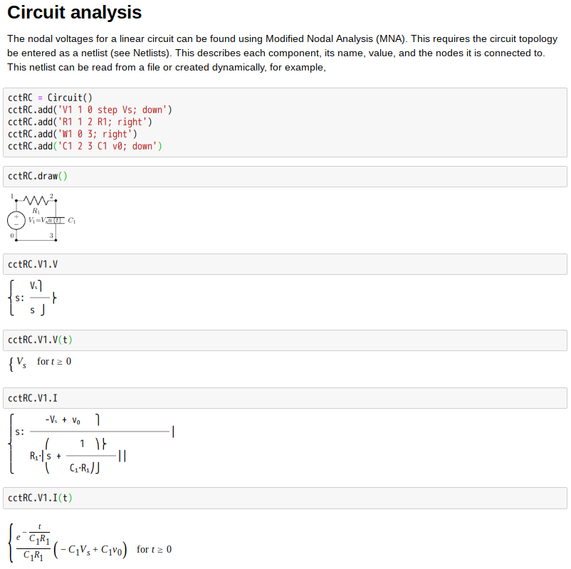
s-domain equivalent circuits and impedances

The Laplace transform is often used in circuit analysis, and simple conversions to the $s$ -domain of circuit elements can be made. Circuit elements can be transformed into impedances, very similar to phasor impedances.

Here is a summary of equivalents:

Note that the resistor is exactly the same in the time domain and the $s$ -domain. The sources are put in if there are initial conditions on the circuit elements. For example, if a capacitor has an initial voltage across it, or if the inductor has an initial current through it, the sources inserted in the $s$ -domain account for that.

The equivalents for current and voltage sources are simply derived from the transformations in the table above.

不過踏腳石也。

欲求論理嚴謹運用從容者，最好能深耕呦︰

The Laplace Transform

Ruye Wang 2012-01-28

倘若還能善使工具，豈非如虎添翼耶☆

※ 參考

【電阻】

$v(t) = i(t) \cdot R$

$\displaystyle {\mathcal {L}}\left\{ v(t) \right\} = \mathcal {L} \left\{ i(t) \right\} \cdot R$

$\therefore \ V(s) = I(s) \cdot R$

【電容】

$i(t) = C \cdot \frac{d \ v(t)}{dt}$

$\displaystyle {\mathcal {L}}\left\{ i(t) \right\} = C \cdot \mathcal {L} \left\{ \frac{d \ v(t)}{dt} \right\}$

$= C \cdot \left( s \cdot \mathcal {L} \left\{ v(t) \right\} - v(0) \right)$

並聯表現︰

$I(s) = \frac{V(s)}{\frac{1}{C \cdot s}} + (- C \cdot v(0))$

串聯表現︰

$V(s) = I(s) \cdot \frac{1}{C \cdot s} + \frac{v(0)}{s}$

【電感】

$v(t) = L \cdot \frac{d \ i(t)}{dt}$

$\displaystyle {\mathcal {L}}\left\{ v(t) \right\} = L \cdot \mathcal {L} \left\{ \frac{d \ i(t)}{dt} \right\}$

$= L \cdot \left( s \cdot \mathcal {L} \left\{ i(t) \right\} - i(0) \right)$

串聯表現︰

$V(s) = I(s) \cdot (L \cdot s) + (- L \cdot i(0) )$

並聯表現︰

$I(s) = \frac{V(s)}{L \cdot s}} + \frac{i(0)}{s}$

Partial fraction decomposition

In algebra, the partial fraction decomposition or partial fraction expansion of a rational function (that is, a fraction such that the numerator and the denominator are both polynomials) is the operation that consists in expressing the fraction as a sum of a polynomial (possibly zero) and one or several fractions with a simpler denominator.

The importance of the partial fraction decomposition lies in the fact that it provides an algorithm for computing the antiderivative of a rational function.^[1] The concept was discovered in 1702 by both Johann Bernoulli and Gottfried Leibniz independently.^[2]

In symbols, one can use partial fraction expansion to change a rational fraction in the form

\displaystyle {\frac {f(x)}{g(x)}}

where f and g are polynomials, into an expression of the form

\displaystyle \sum _{j}{\frac {f_{j}(x)}{g_{j}(x)}}

where g_j (x) are polynomials that are factors of g(x), and are in general of lower degree. Thus, the partial fraction decomposition may be seen as the inverse procedure of the more elementary operation of addition of rational fractions, which produces a single rational fraction with a numerator and denominator usually of high degree. The full decomposition pushes the reduction as far as it can go: in other words, the factorization of g is used as much as possible. Thus, the outcome of a full partial fraction expansion expresses that fraction as a sum of a polynomial and one of several fractions, such that:

the denominator of each fraction is a power of an irreducible (not factorable) polynomial and
the numerator is a polynomial of smaller degree than this irreducible polynomial.

As factorization of polynomials may be difficult, a coarser decomposition is often preferred, which consists of replacing factorization by square-free factorization. This amounts to replace “irreducible” by “square-free” in the preceding description of the outcome.

日	一	二	三	四	五	六
« 6 月				8 月 »
1	2	3	4	5	6	7
8	9	10	11	12	13	14
15	16	17	18	19	20	21
22	23	24	25	26	27	28
29	30	31

FreeSandal

每日彙整: 2018-07-21

STEM 隨筆︰古典力學︰轉子【五】《電路學》四【電容】III

Laplace transform

History

Formal definition

s-domain equivalent circuits and impedances

Partial fraction decomposition

輕。鬆。學。部落客