如何理解『機率母函數』的『定義』呢?
Univariate case
If X is a discrete random variable taking values in the non-negative integers {0,1, …}, then the probability generating function of X is defined as [1]
where p is the probability mass function of X. Note that the subscripted notations GX and pX are often used to emphasize that these pertain to a particular random variable X, and to its distribution. The power series converges absolutely at least for all complex numbers z with |z| ≤ 1; in many examples the radius of convergence is larger.
其實 ![]() ,就是說它是用『隨機變數』
,就是說它是用『隨機變數』 ![]() 在『期望值算符』
在『期望值算符』 ![]() 作用於
作用於 ![]() 下來『定義』的。所以依著『期望值算符』的『定義』
下來『定義』的。所以依著『期望值算符』的『定義』
Univariate discrete random variable, finite case
Suppose random variable X can take value x1 with probability p1, value x2 with probability p2, and so on, up to value xk with probability pk. Then the expectation of this random variable X is defined as
Since all probabilities pi add up to one (p1 + p2 + … + pk = 1), the expected value can be viewed as the weighted average, with pi’s being the weights:
If all outcomes xi are equally likely (that is, p1 = p2 = … = pk), then the weighted average turns into the simple average. This is intuitive: the expected value of a random variable is the average of all values it can take; thus the expected value is what one expects to happen on average. If the outcomes xi are not equally probable, then the simple average must be replaced with the weighted average, which takes into account the fact that some outcomes are more likely than the others. The intuition however remains the same: the expected value of X is what one expects to happen on average.
,得到了 ![]() 這個形式。既與『期望值』相干,期待『數值解析』耶?由於
這個形式。既與『期望值』相干,期待『數值解析』耶?由於 ![]() ,可知
,可知 ![]() 當
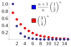
當 ![]() 時皆『收斂』乎??並非『比值審斂法』不足據!
時皆『收斂』乎??並非『比值審斂法』不足據!
Ratio test
In mathematics, the ratio test is a test (or “criterion”) for the convergence of a series
where each term is a real or complex number and an is nonzero when n is large. The test was first published by Jean le Rond d’Alembert and is sometimes known as d’Alembert’s ratio test or as the Cauchy ratio test.[1]
…
The test
The usual form of the test makes use of the limit
-
(1)
The ratio test states that:
- if L < 1 then the series converges absolutely;
- if L > 1 then the series is divergent;
- if L = 1 or the limit fails to exist, then the test is inconclusive, because there exist both convergent and divergent series that satisfy this case.
It is possible to make the ratio test applicable to certain cases where the limit L fails to exist, if limit superior and limit inferior are used. The test criteria can also be refined so that the test is sometimes conclusive even when L = 1. More specifically, let
-
-
.
Then the ratio test states that:[2][3]
- if R < 1, the series converges absolutely;
- if r > 1, the series diverges;
- if
for all large n (regardless of the value of r), the series also diverges; this is because
is nonzero and increasing and hence an does not approach zero;
- the test is otherwise inconclusive.
If the limit L in (1) exists, we must have L = R = r. So the original ratio test is a weaker version of the refined one.
……
Proof
Below is a proof of the validity of the original ratio test.
Suppose that 


That is, the series converges absolutely.
On the other hand, if L > 1, then 
───
,無窮『幾何級數』簡易明!!
Infinite geometric series
An infinite geometric series is an infinite series whose successive terms have a common ratio. Such a series converges if and only if the absolute value of the common ratio is less than one (| r | < 1). Its value can then be computed from the finite sum formulae
Since:
Then:
For a series containing only even powers of 
and for odd powers only,
In cases where the sum does not start at k = 0,
The formulae given above are valid only for | r | < 1. The latter formula is valid in every Banach algebra, as long as the norm of r is less than one, and also in the field of p-adic numbers if | r |p < 1. As in the case for a finite sum, we can differentiate to calculate formulae for related sums. For example,
This formula only works for | r | < 1 as well. From this, it follows that, for | r | < 1,
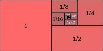
Also, the infinite series 1/2 + 1/4 + 1/8 + 1/16 + ⋯ is an elementary example of a series that converges absolutely.
It is a geometric series whose first term is 1/2 and whose common ratio is 1/2, so its sum is
The inverse of the above series is 1/2 − 1/4 + 1/8 − 1/16 + ⋯ is a simple example of an alternating series that converges absolutely.
It is a geometric series whose first term is 1/2 and whose common ratio is −1/2, so its sum is
Complex numbers
The summation formula for geometric series remains valid even when the common ratio is a complex number. In this case the condition that the absolute value of r be less than 1 becomes that the modulus of r be less than 1. It is possible to calculate the sums of some non-obvious geometric series. For example, consider the proposition
The proof of this comes from the fact that
which is a consequence of Euler’s formula. Substituting this into the original series gives
-
.
This is the difference of two geometric series, and so it is a straightforward application of the formula for infinite geometric series that completes the proof.
故而此『隨機變數』 ![]() 的『期望值』記作
的『期望值』記作 ![]()
Probabilities and expectations
The following properties allow the derivation of various basic quantities related to X:
1. The probability mass function of X is recovered by taking derivatives of G
2. It follows from Property 1 that if random variables X and Y have probability generating functions that are equal, GX = GY, then pX = pY. That is, if X and Y have identical probability generating functions, then they have identical distributions.
3. The normalization of the probability density function can be expressed in terms of the generating function by
The expectation of X is given by
More generally, the kth factorial moment, 
So the variance of X is given by
4. 


,論述邏輯之嚴謹不得不然也!!??

![{\displaystyle \operatorname {E} [X]=x_{1}p_{1}+x_{2}p_{2}+\cdots +x_{k}p_{k}\;.}](https://wikimedia.org/api/rest_v1/media/math/render/svg/998a64bf99a74226d1e0356b69b7c168e3fe3f98)
![\operatorname {E} [X]={\frac {x_{1}p_{1}+x_{2}p_{2}+\dotsb +x_{k}p_{k}}{1}}={\frac {x_{1}p_{1}+x_{2}p_{2}+\dotsb +x_{k}p_{k}}{p_{1}+p_{2}+\dotsb +p_{k}}}\;.](https://wikimedia.org/api/rest_v1/media/math/render/svg/d5a9158e4ef458f8a96a8ae426932fdf35f8d3b1)


![\operatorname {Var} (X)=G''(1^{-})+G'(1^{-})-\left[G'(1^{-})\right]^{2}.](https://wikimedia.org/api/rest_v1/media/math/render/svg/e4e77ce2135d6d93dab77d15b82cda8c60f61779)