若說『成功、失敗』,或講『Yes、No』曾經困惑伯努利因何事?不為『二項式定理』太困難,只為著『二項分佈』之無窮大  的『期望值』!
Binomial distribution
In probability theory and statistics, the binomial distribution with parameters n and p is the discrete probability distribution of the number of successes in a sequence of n independent yes/no experiments, each of which yields success with probability p. A success/failure experiment is also called a Bernoulli experiment or Bernoulli trial; when n = 1, the binomial distribution is a Bernoulli distribution. The binomial distribution is the basis for the popular binomial test of statistical significance.
The binomial distribution is frequently used to model the number of successes in a sample of size n drawn with replacement from a population of size N. If the sampling is carried out without replacement, the draws are not independent and so the resulting distribution is a hypergeometric distribution, not a binomial one. However, for N much larger than n, the binomial distribution remains a good approximation, and is widely used.
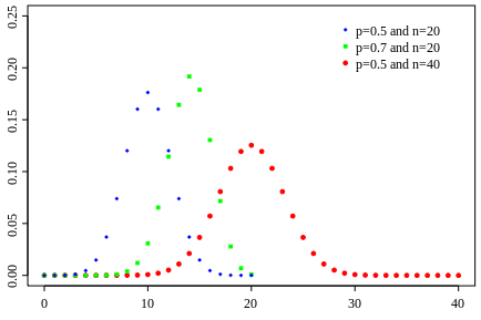
Probability mass function
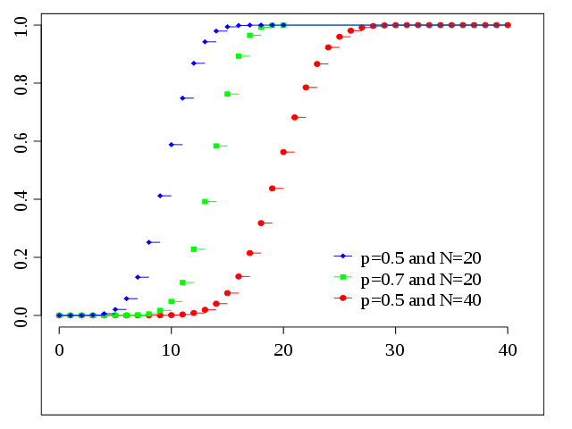
Cumulative distribution function
Specification
Probability mass function
In general, if the random variable X follows the binomial distribution with parameters n ∈ ℕ and p ∈ [0,1], we write X ~ B(n, p). The probability of getting exactly k successes in n trials is given by the probability mass function:

for k = 0, 1, 2, …, n, where

is the binomial coefficient, hence the name of the distribution. The formula can be understood as follows. k successes occur with probability pk and n − k failures occur with probability (1 − p)n − k. However, the k successes can occur anywhere among the n trials, and there are 
In creating reference tables for binomial distribution probability, usually the table is filled in up to n/2 values. This is because for k > n/2, the probability can be calculated by its complement as

The probability mass function satisfies the following recurrence relation, for every 
![\left\{{\begin{array}{l}p(n-k)f(k,n,p)=(k+1)(1-p)f(k+1,n,p),\\[10pt]f(0,n,p)=(1-p)^{n}\end{array}}\right\}](https://wikimedia.org/api/rest_v1/media/math/render/svg/9512786caa7fe137b26b2c5d7b504fdfe111ea82)
Looking at the expression ƒ(k, n, p) as a function of k, there is a k value that maximizes it. This k value can be found by calculating

and comparing it to 1. There is always an integer M that satisfies

ƒ(k, n, p) is monotone increasing for k < M and monotone decreasing for k > M, with the exception of the case where (n + 1)p is an integer. In this case, there are two values for which ƒ is maximal: (n + 1)p and (n + 1)p − 1. M is the most probable (most likely) outcome of the Bernoulli trials and is called the mode. Note that the probability of it occurring can be fairly small.

Binomial distribution for
with n and k as in Pascal’s triangle

The probability that a ball in a Galton box with 8 layers (n = 8) ends up in the central bin (k = 4) is 
莫言『機率』百分百未必然,『無窮大』尚可以分等級。且用二項分布之『生成函數』 


【※ 註︰當然此處取  。】
。】
談談它的『期望值』之推導
 。可知無論『成功率』
  有多小,當
有多小,當  時,必然是趨近無窮大 矣。
事實上它的『方差』 

 也是無窮大的哩。
故算術的簡單與否、形式之自動也罷,論及理解如之何哉︰
假使仔細觀察與比較用『德汝德模型』來推導『歐姆定律』,這是電子的『動量傳輸』現象  ,來自於
,來自於  到
到  間不發生『碰撞』的電子;當論述『焦耳定律』時,這又是電子的『能量移轉』現象
  ,發生在 到 間與『正離子』發生『碰撞』的電子。這兩個現象同時而起,各自『電場』中汲取『動量』和『能量』。為了更深入的理解,就讓我們稍微談一談『機率』與『統計』吧!
擲一個硬幣產生『正‧反』面兩種結果,這是很普通的現象,今天在『術語』上稱之為『伯努利試驗』Bernoulli trial,是說對一個只有兩種可能結果的單次『隨機試驗』,就一個『隨機變數』  而言,
而言,
![Pr[X = 1] \ = \ p](http://www.freesandal.org/wp-content/ql-cache/quicklatex.com-9343f7df370d1e51787a88d7cdff18ed_l3.png "Rendered by QuickLaTeX.com")
![Pr[X = 0] \ = \ 1-p = q](http://www.freesandal.org/wp-content/ql-cache/quicklatex.com-dec4972a4a8e92da1fdb6a1e6c810d82_l3.png "Rendered by QuickLaTeX.com")
,此處 ![{Pr}_i[X_i = {\alpha}_i] = q_i](http://www.freesandal.org/wp-content/ql-cache/quicklatex.com-6f2da4060b11a0529c27c1ece41cfab5_l3.png "Rendered by QuickLaTeX.com") 是說『隨機變數』
是說『隨機變數』  有
有  的機會取
的機會取  的值。從『期望值』的角度講

,它的『標準差』 Standard Deviation 是

。這為什麼要叫做『伯努利試驗』的呢?一七三零年代,荷蘭出生大部分時間居住在瑞士巴塞爾的丹尼爾‧伯努利 Daniel Bernoulli 之堂兄尼古拉一世‧伯努利 Nikolaus I. Bernoulli,在致法國數學家皮耶‧黑蒙‧德蒙馬特 Pierre Rémond de Montmort 的信件中,提出了一個問題:擲 一枚硬幣,假使第一次擲出正面,你就賺了  元。如果第一次出現反面,那就要再擲一次,若是第二次擲的是正面,你便賺了
  元。要是第二次擲出反面,那就得要擲第三次,假若第三次擲的是正面,你便賺
  元……如此類推,也就是說你可能擲一次遊戲就結束了,也許會反覆擲個沒完沒了。問題是,你最多肯付多少錢來玩這個遊戲的呢?假使從『期望值』來考量,這個遊戲的期望值是『無限大』


,然而即使你願意付出『無限的金錢』去參與這個遊戲。不過,你卻可能只賺到 元,或 元,或  元……等等,只怕不可能賺到無限的金錢。那你又為什麼肯付出巨額的金錢加入遊戲的呢?
其後丹尼爾‧白努利於一七三八年寫了一篇論文『風險度量的新理論之討論』考慮了一個對等的遊戲,不斷的擲同一枚硬幣,直到獲得正面為止,如果你擲了  次才最終得到正面,你將獲得
  元。即使參與玩這個遊戲的花費是『天價』,假使我們考慮到這個遊戲的『期望收益』是無窮大,我們就應該參加。這就是史稱的『聖彼得堡悖論』。白努利提出了一個理論來解釋這個悖論,他得到了一條原理,『財富越多人越滿足,然而隨著財富的累積,滿足程度的增加率卻不斷下降』。這或許可以說是古典的『邊際效用遞減』版本,就像『白手起家』和其後之『錦上添花』,對一個人的『效用』之『滿足』是完全不同的一樣。他這麼講︰
【邊際效用遞減原理】:一個人對於財富的佔有多多益善,就是說『效用函數』一階導數大於零;隨著財富的增加,滿足程度的增加速度不斷下降,正因為『效用函數』二階導數小於零。
【最大效用原理】:在『風險』和『不確定』的條件下,一個人行為的『決策準則』是為了獲得最大『期望效用』值而不是最大『期望金額』值。
作者不知『理性』是否該『相信』期望值,或者『感性』果就會『追求』效用量,彷彿『天下』到底是『患寡』還是『患不均』的呢??
事實上一個『發生』或『不發生』,『存在』也許『不存在』,是『成功』還是『失敗』的『可‧不可』 Yes or No 的『事件機率』能夠表達的『現象界』不勝枚舉,就像『德汝德模型』中『電子』之『碰撞』與『不碰撞』也是一樣的。假使我們將『伯努利試驗』推廣到  次中有
次中有  次的『成功率』,我們就得到了數學上所謂的『二項分佈』

,此處  是 中取 之『組合數』。假使 很大,且機率 很小,這個『二項分佈』可以『近似』如下︰
如果  是有限大小的『適度量』,回顧指數函數
  的定義之一是

依據二項分佈的定義:

如果假設  ,當 趨於無窮時,
  的極限可以如此計算


![=\lim \limits_{n\to\infty} \underbrace{\left[\frac{n!}{n^k\left(n-k\right)!}\right]}_F \left(\frac{\lambda^k}{k!}\right) \underbrace{\left(1-\frac{\lambda}{n}\right)^n}_{\to\exp\left(-\lambda\right)} \underbrace{\left(1-\frac{\lambda}{n}\right)^{-k}}_{\to 1}](http://www.freesandal.org/wp-content/ql-cache/quicklatex.com-f16abcae54bf5047a0eea7c5c1b79a53_l3.png "Rendered by QuickLaTeX.com")
![= \lim \limits_{n\to\infty} \underbrace{\left[ \left(1-\frac{1}{n}\right)\left(1-\frac{2}{n}\right) \ldots \left(1-\frac{k-1}{n}\right) \right]}_{\to 1} \left(\frac{\lambda^k}{k!}\right) \underbrace{\left(1-\frac{\lambda}{n}\right)^n}_{\to\exp\left(-\lambda\right)} \underbrace{\left(1-\frac{\lambda}{n}\right)^{-k}}_{\to 1}](http://www.freesandal.org/wp-content/ql-cache/quicklatex.com-f9a1ceb4a6c8ec5597d00366fd3a1e11_l3.png "Rendered by QuickLaTeX.com")
 。
。
─── 摘自《【Sonic π】電路學之補充《一》》