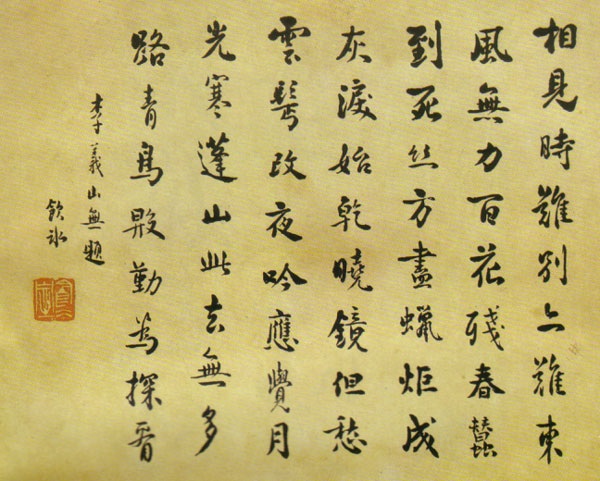
梁啟超手書李商隱無題詩

唐‧李商隱‧無題二首之一

昨夜星辰昨夜風，畫樓西畔桂堂東。
身無彩鳳雙飛翼，心有靈犀一點通。
隔座送鉤春酒暖，分曹射覆蠟燈紅。
嗟余聽鼓應官去，走馬蘭台類轉蓬。

之二

聞道閶門萼綠華，昔年相望抵天涯。
豈知一夜秦樓客，偷看吳王苑內花。

昨夜何必候風觀星辰？今宵誰人畫樓桂堂中？心有身無什麼幽情？靈犀彩鳳全得能成？送鉤射覆春夜遊戲？隔座分曹燈紅比鄰？此日方聽鼓走馬藍台耶？？怎不嗟余應官類轉蓬乎！！

史學大師陳寅恪先生說以『詩文證史』難矣哉！試想如果字詞聲韻所知不多，欣賞都不容易，能夠訓詁證史乎？不過好詩詞讀來丁丁冬冬，意境優美彷彿意有所指，偶爾夢回聽鼓之際，一時恍惚忽而睹見，焉知不會心有靈犀一點通耶？？

如是怎麼從已被陳述之公式、定理、命題，還原想法、思路之歷史由來呢？？！！所以講關聯之重要以及同理之難得矣！！？？即使不知萊布尼茨與 π 故事的前後次序，只是並排列舉那些相關詞條

Leibniz formula for $π$

In mathematics, the Leibniz formula for $π$ , named after Gottfried Leibniz , states that

1\,-\,{\frac {1}{3}}\,+\,{\frac {1}{5}}\,-\,{\frac {1}{7}}\,+\,{\frac {1}{9}}\,-\,\cdots \,=\,{\frac {\pi }{4}}.

It is also called Madhava–Leibniz series as it is a special case of a more general series expansion for the inverse tangent function, first discovered by the Indian mathematician Madhava of Sangamagrama in the 14th century. The series for the inverse tangent function, which is also known as Gregory’s series, can be given by:

\arctan x=x-{\frac {x^{3}}{3}}+{\frac {x^{5}}{5}}-{\frac {x^{7}}{7}}+\cdots

The Leibniz formula for $π$ /4 can be obtained by plugging $x = 1$ into the above inverse-tangent series.^[1]

It also is the Dirichlet $L$ -series of the non-principal Dirichlet character of modulus 4 evaluated at $s = 1$ , and therefore the value $β (1)$ of the Dirichlet beta function.

Proof

{\begin{aligned}{\frac {\pi }{4}}&=\arctan(1)\\&=\int _{0}^{1}{\frac {1}{1+x^{2}}}\,dx\\[8pt]&=\int _{0}^{1}\left(\sum _{k=0}^{n}(-1)^{k}x^{2k}+{\frac {(-1)^{n+1}\,x^{2n+2}}{1+x^{2}}}\right)\,dx\\[8pt]&=\left(\sum _{k=0}^{n}{\frac {(-1)^{k}}{2k+1}}\right)+(-1)^{n+1}\left(\int _{0}^{1}{\frac {x^{2n+2}}{1+x^{2}}}\,dx\right).\end{aligned}}

Considering only the integral in the last line, we have:

0<\int _{0}^{1}{\frac {x^{2n+2}}{1+x^{2}}}\,dx<\int _{0}^{1}x^{2n+2}\,dx={\frac {1}{2n+3}}\;\rightarrow 0{\text{ as }}n\rightarrow \infty .

Therefore, by the squeeze theorem, as $n \to \infty$ we are left with the Leibniz series:

{\frac {\pi }{4}}=\sum _{k=0}^{\infty }{\frac {(-1)^{k}}{2k+1}}

For a more detailed proof, together with the original geometric proof by Leibniz himself, see Leibniz’s Formula for Pi.^[2]

Inverse trigonometric functions

Infinite series

Like the sine and cosine functions, the inverse trigonometric functions can be calculated using power series, as follows. For arcsine, the series can be derived by expanding its derivative, ${\frac {1}{\sqrt {1-z^{2}}}}$ , as a binomial series, and integrating term by term (using the integral definition as above). The series for arctangent can similarly be derived by expanding its derivative ${\frac {1}{1+z^{2}}}$ in a geometric series and applying the integral definition above (see Leibniz series).

\arcsin(z)=z+\left({\frac {1}{2}}\right){\frac {z^{3}}{3}}+\left({\frac {1\cdot 3}{2\cdot 4}}\right){\frac {z^{5}}{5}}+\left({\frac {1\cdot 3\cdot 5}{2\cdot 4\cdot 6}}\right){\frac {z^{7}}{7}}+\cdots =\sum _{n=0}^{\infty }{\frac {(2n-1)!!}{(2n)!!}}\cdot {\frac {z^{2n+1}}{2n+1}}=\sum _{n=0}^{\infty }{\frac {{\binom {2n}{n}}z^{2n+1}}{4^{n}(2n+1)}}\,;\qquad |z|\leq 1

\arctan(z)=z-{\frac {z^{3}}{3}}+{\frac {z^{5}}{5}}-{\frac {z^{7}}{7}}+\cdots =\sum _{n=0}^{\infty }{\frac {(-1)^{n}z^{2n+1}}{2n+1}}\,;\qquad |z|\leq 1\qquad z\neq i,-i

Series for the other inverse trigonometric functions can be given in terms of these according to the relationships given above. For example, $\arccos x=\pi /2-\arcsin x$ , $\operatorname {arccsc} x=\arcsin(1/x)$ , and so on. Another series is given by:

2\left(\arcsin {\frac {x}{2}}\right)^{2}=\sum _{n=1}^{\infty }{\frac {x^{2n}}{n^{2}{\binom {2n}{n}}}}

^[7]

Leonhard Euler found a more efficient series for the arctangent, which is:

\arctan(z)={\frac {z}{1+z^{2}}}\sum _{n=0}^{\infty }\prod _{k=1}^{n}{\frac {2kz^{2}}{(2k+1)(1+z^{2})}}\,.

(Notice that the term in the sum for n = 0 is the empty product which is 1.)
Alternatively, this can be expressed:

\arctan z=\sum _{n=0}^{\infty }{\frac {2^{2n}(n!)^{2}}{(2n+1)!}}\;{\frac {z^{2n+1}}{(1+z^{2})^{n+1}}}

Alternating series test

In mathematical analysis, the alternating series test is the method used to prove that an alternating series with terms that decrease in absolute value is a convergent series. The test was used by Gottfried Leibniz and is sometimes known as Leibniz’s test, Leibniz’s rule, or the Leibniz criterion.

Formulation

A series of the form

\sum _{n=0}^{\infty }(-1)^{n}a_{n}=a_{0}-a_{1}+a_{2}-a_{3}+\cdots \!

where either all a_n are positive or all a_n are negative, is called an alternating series.

The alternating series test then says: if $|a_n|$ decreases monotonically and $\lim _{{n\to \infty }}a_{n}=0$ then the alternating series converges.

Moreover, let L denote the sum of the series, then the partial sum

S_k = \sum_{n=1}^k (-1)^{n-1} a_n\!

approximates L with error bounded by the next omitted term:

\left | S_k - L \right \vert \le \left | S_k - S_{k+1} \right \vert = a_{k+1}.\!

果不能斷言萊布尼茨已知 $\frac{\pi}{4} = 1 - \frac{1}{3} + \frac{1}{5} - \frac{1}{7} + \cdots$ 乎？說不定他也知 $\frac{\pi}{8} = \frac{1}{1 \cdot 3} + \frac{1}{5 \cdot 7} + \cdots$ ，還知 $1 - \frac{\pi}{8} = \frac{1}{3 \cdot 5} + \frac{1}{7 \cdot 9} + \cdots$ 哩！

那麼能否推論歐拉不只讀過萊布尼茨的著作，尚且看過

Vieta’s formulas

In mathematics, Vieta’s formulas are formulas that relate the coefficients of a polynomial to sums and products of its roots. Named after François Viète (more commonly referred to by the Latinised form of his name, Franciscus Vieta), the formulas are used specifically in algebra.

The laws

Basic formulas

Any general polynomial of degree n

P(x)=a_{n}x^{n}+a_{n-1}x^{n-1}+\cdots +a_{1}x+a_{0}\,

(with the coefficients being real or complex numbers and a_n ≠ 0) is known by the fundamental theorem of algebra to have n (not necessarily distinct) complex roots x₁, x₂, …, x_n. Vieta’s formulas relate the polynomial’s coefficients { a_k } to signed sums and products of its roots { x_i } as follows:

{\begin{cases}x_{1}+x_{2}+\dots +x_{n-1}+x_{n}=-{\dfrac {a_{n-1}}{a_{n}}}\\(x_{1}x_{2}+x_{1}x_{3}+\cdots +x_{1}x_{n})+(x_{2}x_{3}+x_{2}x_{4}+\cdots +x_{2}x_{n})+\cdots +x_{n-1}x_{n}={\dfrac {a_{n-2}}{a_{n}}}\\{}\quad \vdots \\x_{1}x_{2}\dots x_{n}=(-1)^{n}{\dfrac {a_{0}}{a_{n}}}.\end{cases}}

Equivalently stated, the (n − k)th coefficient a_n−k is related to a signed sum of all possible subproducts of roots, taken k-at-a-time:

\sum _{1\leq i_{1}<i_{2}<\cdots <i_{k}\leq n}x_{i_{1}}x_{i_{2}}\cdots x_{i_{k}}=(-1)^{k}{\frac {a_{n-k}}{a_{n}}}

for k = 1, 2, …, n (where we wrote the indices i_k in increasing order to ensure each subproduct of roots is used exactly once).

The left hand sides of Vieta’s formulas are the elementary symmetric functions of the roots.

……

Newton’s identities

In mathematics, Newton’s identities, also known as the Newton–Girard formulae, give relations between two types of symmetric polynomials, namely between power sums and elementary symmetric polynomials. Evaluated at the roots of a monic polynomial P in one variable, they allow expressing the sums of the k-th powers of all roots of P (counted with their multiplicity) in terms of the coefficients of P, without actually finding those roots. These identities were found by Isaac Newton around 1666, apparently in ignorance of earlier work (1629) by Albert Girard. They have applications in many areas of mathematics, including Galois theory, invariant theory, group theory, combinatorics, as well as further applications outside mathematics, including general relativity.

Mathematical statement

Formulation in terms of symmetric polynomials

Let x₁, …, x_n be variables, denote for k ≥ 1 by p_k(x₁, …, x_n) the k-th power sum:

p_{k}(x_{1},\ldots ,x_{n})=\sum \nolimits _{i=1}^{n}x_{i}^{k}=x_{1}^{k}+\cdots +x_{n}^{k},

and for k ≥ 0 denote by e_k(x₁, …, x_n) the elementary symmetric polynomial (that is, the sum of all distinct products of k distinct variables), so

{\begin{aligned}e_{0}(x_{1},\ldots ,x_{n})&=1,\\e_{1}(x_{1},\ldots ,x_{n})&=x_{1}+x_{2}+\cdots +x_{n},\\e_{2}(x_{1},\ldots ,x_{n})&=\textstyle \sum _{1\leq i<j\leq n}x_{i}x_{j},\\e_{n}(x_{1},\ldots ,x_{n})&=x_{1}x_{2}\cdots x_{n},\\e_{k}(x_{1},\ldots ,x_{n})&=0,\quad {\text{for}}\ k>n.\\\end{aligned}}

Then Newton’s identities can be stated as

ke_{k}(x_{1},\ldots ,x_{n})=\sum _{i=1}^{k}(-1)^{i-1}e_{k-i}(x_{1},\ldots ,x_{n})p_{i}(x_{1},\ldots ,x_{n}),

valid for all n ≥ 1 and k ≥ 1.

Also, one has

0=\sum _{i=k-n}^{k}(-1)^{i-1}e_{k-i}(x_{1},\ldots ,x_{n})p_{i}(x_{1},\ldots ,x_{n}),

for all k > n ≥ 1.

Concretely, one gets for the first few values of k:

{\begin{aligned}e_{1}(x_{1},\ldots ,x_{n})&=p_{1}(x_{1},\ldots ,x_{n}),\\2e_{2}(x_{1},\ldots ,x_{n})&=e_{1}(x_{1},\ldots ,x_{n})p_{1}(x_{1},\ldots ,x_{n})-p_{2}(x_{1},\ldots ,x_{n}),\\3e_{3}(x_{1},\ldots ,x_{n})&=e_{2}(x_{1},\ldots ,x_{n})p_{1}(x_{1},\ldots ,x_{n})-e_{1}(x_{1},\ldots ,x_{n})p_{2}(x_{1},\ldots ,x_{n})+p_{3}(x_{1},\ldots ,x_{n}).\\\end{aligned}}

The form and validity of these equations do not depend on the number n of variables (although the point where the left-hand side becomes 0 does, namely after the n-th identity), which makes it possible to state them as identities in the ring of symmetric functions. In that ring one has

{\begin{aligned}e_{1}&=p_{1},\\2e_{2}&=e_{1}p_{1}-p_{2},\\3e_{3}&=e_{2}p_{1}-e_{1}p_{2}+p_{3},\\4e_{4}&=e_{3}p_{1}-e_{2}p_{2}+e_{1}p_{3}-p_{4},\\\end{aligned}}

and so on; here the left-hand sides never become zero. These equations allow to recursively express the e_i in terms of the p_k; to be able to do the inverse, one may rewrite them as

{\begin{aligned}p_{1}&=e_{1},\\p_{2}&=e_{1}p_{1}-2e_{2},\\p_{3}&=e_{1}p_{2}-e_{2}p_{1}+3e_{3},\\p_{4}&=e_{1}p_{3}-e_{2}p_{2}+e_{3}p_{1}-4e_{4},\\&{}\ \ \vdots \end{aligned}}

In general, we have

p_{k}(x_{1},\ldots ,x_{n})=(-1)^{k-1}ke_{k}(x_{1},\ldots ,x_{n})+\sum _{i=1}^{k-1}(-1)^{k-1+i}e_{k-i}(x_{1},\ldots ,x_{n})p_{i}(x_{1},\ldots ,x_{n}),

valid for all n ≥ 1 and k ≥ 1.

Also, one has

p_{k}(x_{1},\ldots ,x_{n})=\sum _{i=k-n}^{k-1}(-1)^{k-1+i}e_{k-i}(x_{1},\ldots ,x_{n})p_{i}(x_{1},\ldots ,x_{n}),

for all k > n ≥ 1.

Application to the roots of a polynomial

The polynomial with roots x_i may be expanded as

\prod _{i=1}^{n}\left(x-x_{i}\right)=\sum _{k=0}^{n}(-1)^{n+k}e_{n-k}x^{k},

where the coefficients $e_{k}(x_{1},\ldots ,x_{n})$ are the symmetric polynomials defined above. Given the power sums of the roots

p_{k}(x_{1},\ldots ,x_{n})=\sum _{i=1}^{n}x_{i}^{k},

the coefficients of the polynomial with roots $x_{1},\ldots ,x_{n}$ may be expressed recursively in terms of the power sums as

{\begin{aligned}e_{0}&=1,\\e_{1}&=p_{1},\\e_{2}&={\frac {1}{2}}(e_{1}p_{1}-p_{2}),\\e_{3}&={\frac {1}{3}}(e_{2}p_{1}-e_{1}p_{2}+p_{3}),\\e_{4}&={\frac {1}{4}}(e_{3}p_{1}-e_{2}p_{2}+e_{1}p_{3}-p_{4}),\\&{}\ \ \vdots \end{aligned}}

Formulating polynomial this way is useful in using the method of Delves and Lyness^[1] to find the zeros of an analytic function.

呀？？突然心領神會，一日飛來之筆，於是用

假設 $y = \sin(x)$ ，所以 $\frac{\sin(x)}{y} = 1$ ，因此 $0 = 1 - \frac{\sin(x)}{y}$ $= 1 - \frac{x}{y} + \frac{x^3}{3! y} - \frac{x^5}{5! y} + \cdots$ 。

如果 $A$ 是滿足 $\sin(A) = y$ 的最小正值，那麼 $A + 2 n \pi$ 與 $-\pi - A + 2 n \pi$ 都是其根。根之因子式就可以表示為

$0 = \left( 1 - \frac{x}{A} \right) \left( 1 - \frac{x}{- \pi - A} \right) \cdots$

將兩種無限代數表達式關聯起來，這等奇怪思路也！！

講借著牛頓恆等式推導根之多次倒數和

$\frac{1}{A} + \frac{1}{\pi -A} + \frac{1}{2 \pi +A} + \cdots - \frac{1}{\pi + A} - \frac{1}{2 \pi - A} - \frac{1}{3 \pi + A} - \cdots = \frac{1}{y}$

$\frac{1}{A^2} + \frac{1}{{(\pi -A)}^2} + \frac{1}{{(2 \pi +A)}^2} + \cdots + \frac{1}{{(\pi + A)}^2} + \frac{1}{{(2 \pi - A)}^2} - \frac{1}{{(3 \pi + A)}^2} + \cdots = \frac{1}{y^2}$

$\cdots$

難道不是創舉嗎？若說只取

$\sin(\frac{\pi}{2}}) = 1$ ，計算出

$\frac{\pi}{4} = 1 - \frac{1}{3} + \frac{1}{5} - \frac{1}{7} + \cdots$

$\frac{{\pi}^2}{8} = 1 + \frac{1}{3^2} + \frac{1}{5^2} + \frac{1}{7^2} + \cdots$

……

就以為得到了要旨！！怕是尚未明白數學方法和精神的吧？？

日	一	二	三	四	五	六
« 2 月				4 月 »
			1	2	3	4
5	6	7	8	9	10	11
12	13	14	15	16	17	18
19	20	21	22	23	24	25
26	27	28	29	30	31

FreeSandal

每日彙整: 2017-03-30

時間序列︰生成函數‧漸近展開︰白努利 □○《九中》