此處 Michael Nielsen 先生談起『理論』上可行的方法,『實務』上可能會不管用!!??
People have investigated many variations of gradient descent, including variations that more closely mimic a real physical ball. These ball-mimicking variations have some advantages, but also have a major disadvantage: it turns out to be necessary to compute second partial derivatives of  , and this can be quite costly. To see why it’s costly, suppose we want to compute all the second partial derivatives
  . If there are a million such
  variables then we’d need to compute something like a trillion (i.e., a million squared) second partial derivatives*
*Actually, more like half a trillion, since  . Still, you get the point.!
That’s going to be computationally costly. With that said, there are tricks for avoiding this kind of problem, and finding alternatives to gradient descent is an active area of investigation. But in this book we’ll use gradient descent (and variations) as our main approach to learning in neural networks.
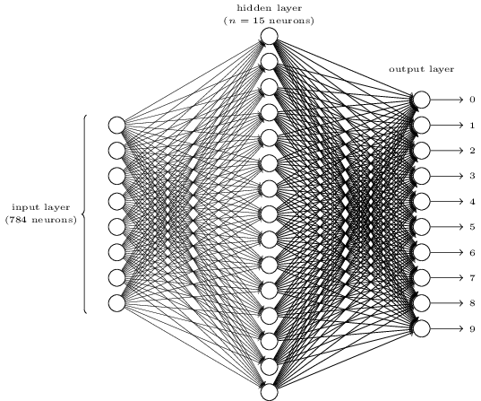
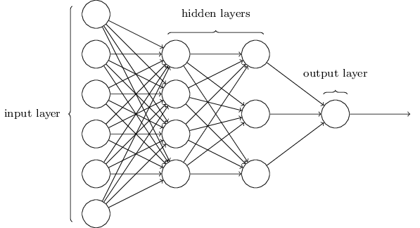
How can we apply gradient descent to learn in a neural network? The idea is to use gradient descent to find the weights wk and biases bl which minimize the cost in Equation (6). To see how this works, let’s restate the gradient descent update rule, with the weights and biases replacing the variables . In other words, our “position” now has components  and
and  , and the gradient vector
  has corresponding components
  and
and  . Writing out the gradient descent update rule in terms of components, we have

 .
.
By repeatedly applying this update rule we can “roll down the hill”, and hopefully find a minimum of the cost function. In other words, this is a rule which can be used to learn in a neural network.
There are a number of challenges in applying the gradient descent rule. We’ll look into those in depth in later chapters. But for now I just want to mention one problem. To understand what the problem is, let’s look back at the quadratic cost in Equation (6). Notice that this cost function has the form  , that is, it’s an average over costs
  for individual training examples. In practice, to compute the gradient we need to compute the gradients
  separately for each training input,
  , and then average them,
  . Unfortunately, when the number of training inputs is very large this can take a long time, and learning thus occurs slowly.
An idea called stochastic gradient descent can be used to speed up learning. The idea is to estimate the gradient by computing for a small sample of randomly chosen training inputs. By averaging over this small sample it turns out that we can quickly get a good estimate of the true gradient , and this helps speed up gradient descent, and thus learning.
………
什麼是『隨機』呢?維基百科詞條這麼說︰
Stochastic
The term stochastic occurs in a wide variety of professional or academic fields to describe events or systems that are unpredictable due to the influence of a random variable. The word “stochastic” comes from the Greek word στόχος (stokhos, “aim”).
Researchers refer to physical systems in which they are uncertain about the values of parameters, measurements, expected input and disturbances as “stochastic systems”. In probability theory, a purely stochastic system is one whose state is randomly determined, having a random probability distribution or pattern that may be analyzed statistically but may not be predicted precisely. In this regard, it can be classified as non-deterministic (i.e., “random”) so that the subsequent state of the system is determined probabilistically. Any system or process that must be analyzed using probability theory is stochastic at least in part.[1][2] Stochastic systems and processes play a fundamental role in mathematical models of phenomena in many fields of science, engineering, finance and economics.
───
或可嘗試進一步了解︰
Stochastic gradient descent
Stochastic gradient descent (often shortened in SGD) is a stochastic approximation of the gradient descent optimization method for minimizing an objective function that is written as a sum of differentiable functions.
Iterative method
In stochastic (or “on-line”) gradient descent, the true gradient of  is approximated by a gradient at a single example:

As the algorithm sweeps through the training set, it performs the above update for each training example. Several passes can be made over the training set until the algorithm converges. If this is done, the data can be shuffled for each pass to prevent cycles. Typical implementations may use an adaptive learning rate so that the algorithm converges.
In pseudocode, stochastic gradient descent can be presented as follows:
- Choose an initial vector of parameters
 and learning rate
  .
. - Repeat until an approximate minimum is obtained:
- Randomly shuffle examples in the training set.
- For
 , do:
, do:

A compromise between computing the true gradient and the gradient at a single example, is to compute the gradient against more than one training example (called a “mini-batch”) at each step. This can perform significantly better than true stochastic gradient descent because the code can make use of vectorization libraries rather than computing each step separately. It may also result in smoother convergence, as the gradient computed at each step uses more training examples.
The convergence of stochastic gradient descent has been analyzed using the theories of convex minimization and of stochastic approximation. Briefly, when the learning rates decrease with an appropriate rate, and subject to relatively mild assumptions, stochastic gradient descent converges almost surely to a global minimum when the objective function is convex or pseudoconvex, and otherwise converges almost surely to a local minimum.[3] [4] This is in fact a consequence of the Robbins-Siegmund theorem.[5]
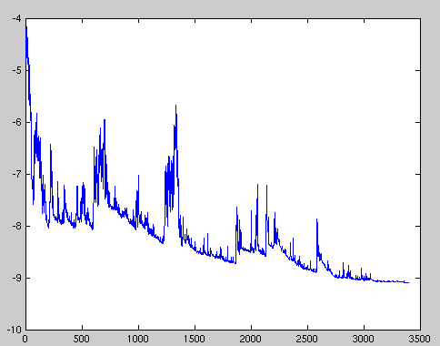
Fluctuations in the total objective function as gradient steps with respect to mini-batches are taken.
───
或可藉『統計力學』揣想它之『合理性』可能有根源耶??!!
假使我們思考這樣的一個『問題』︰
一個由大量粒子構成的『物理系統』,這些粒子具有某一個『物理過程』描述的『隨機變量』  ,那麼在
,那麼在  時刻,這個『隨機變量』的『大數平均值』
![\frac{1}{N} \sum \limits_{i=1}^{N} P[X = X_i] \cdot X_i](http://www.freesandal.org/wp-content/ql-cache/quicklatex.com-95bc83c4e1c59764865f06e8710637d8_l3.png "Rendered by QuickLaTeX.com")
,是這個『物理系統』由大量粒子表現的『瞬時圖像』,也就是『統計力學』上所說的『系綜平均』ensemble average 值。再從一個『典型粒子』的『隨機運動』上講,這個『隨機變量』  會在不同時刻隨機的取值,因此就可以得到此一個『典型粒子』之『隨機變量』的『時間平均值』
![\frac{1}{N} \sum \limits_{i=1}^{N} P[t = t_i] \cdot X_{this}(t_i)](http://www.freesandal.org/wp-content/ql-cache/quicklatex.com-8b9bdc05082726bee30ed0364b816ed6_l3.png "Rendered by QuickLaTeX.com")
,這說明了此一『典型粒子』在『物理系統』中的『歷時現象』 ,那麼此兩種平均值,它們的大小是一樣的嗎??
在『德汝德模型』中我們已經知道  是一個『電子』於 時距裡不發生碰撞的機率。這樣
  的意思就是,在 到
  的時間點發生碰撞的機率。參考指數函數
  的『泰勒展開式』

,如此
![P_{nc}(t) - P_{nc}(t+dt) = e^{- \frac {t}{ \tau}} - e^{- \frac {t+dt}{ \tau}} = e^{- \frac {t}{ \tau}} \left[ 1 - e^{- \frac {dt}{ \tau}} \right]](http://www.freesandal.org/wp-content/ql-cache/quicklatex.com-6021493baa5bc2bdbbd739993a7ab8e2_l3.png "Rendered by QuickLaTeX.com")

,這倒過來說明了為什麼在『德汝德模型』中,發生碰撞的機率是  ,於是一個有
  個『自由電子』的導體,在 時刻可能有
  個電子發生碰撞,碰撞『平均時距』的『系綜平均』是

。比之於《【Sonic π】電路學之補充《一》》一文中之電子的『時間平均值』,果然這兩者相等。事實上一般物理系統要是處於統計力學所說的『平衡狀態』,這兩種『平均值』都會是『相等』的。當真是『考典範以歷史』與『察大眾於一時』都能得到相同結論的嗎??
─── 摘自《【Sonic π】電路學之補充《二》》


 .
.


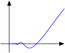
 . So gradient descent can be viewed as a way of taking small steps in the direction which does the most to immediately decrease
  在點
在點 處
處 下降最快。
下降最快。
 為一個夠小數值時成立,那麼
 。
。 的局部極小值的初始估計
 出發,並考慮如下序列
  使得
使得 。
。
 收斂到期望的極值。注意每次疊代步長
 可以改變。
可以改變。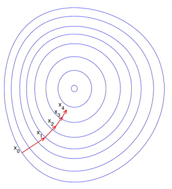

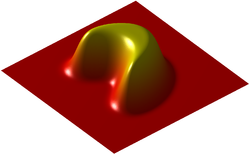
 處,數值為
處,數值為 。但是此函數具有狹窄彎曲的山谷,最小值
 ,速度為
,速度為  時。這時粒子的動量為
  ,當乘以此無窮小距離
  ,這是粒子的動量作用於無窮小『路徑』
  為最小值的『路徑』;如果假定質量是個常數,也就是
 為最小值的『軌道』。
 之中, 粒子所選擇的『路徑』是『作用量』
 泛函數的『極值』,這是牛頓第二運動定律的『變分法』Variation 描述。如果從今天物理能量的觀點來看
  ,此處
,此處  就是粒子的動能。因為牛頓第二運動定律可以表述為
  ,所以
,所以  。
。 ,於是如果一個粒子在一個保守場中,
 ,這就是物理上『能量守恆』原理!舉例來說重力、彈簧力、電場力等等,都是保守力,然而摩擦力和空氣阻力種種都是典型的非保守力。由於
  在這些可能路徑裡都不變,因此『最小作用量原理』所確定的『路徑』也就是『作用量』
  的『極值』。一七八八年法國籍義大利裔數學家和天文學家約瑟夫‧拉格朗日 Joseph Lagrange 對於變分法發展貢獻很大,最早在其論文《分析力學》Mecanique Analytique 裡,使用『能量守恆定律』推導出了歐拉陳述的最小作用量原理的正確性。
 就像『結果
就像『結果  原因』描繪『因果』的『瞬刻聯繫』關係,這是一種『決定論』,從一個『時空點』推及『無窮小時距』
  接續的另一個『時空點』,因此一旦知道『初始狀態』,就已經確定了它的『最終結局』!有人講
  彷彿確定了『目的地』無論從哪個『起始處』出發,總會有一個『通達路徑』,這成了一種『目的論』,大自然自會找到『此時此處』通向『彼時彼處』的『道路』!!
 ,則
,則![\varphi\left(\mathbf{q}\right)-\varphi\left(\mathbf{p}\right) = \int_{\gamma[\mathbf{p},\,\mathbf{q}]} \nabla\varphi(\mathbf{r})\cdot d\mathbf{r}.](https://upload.wikimedia.org/math/c/a/8/ca8b2c89c9693e534bf73ab7c65d411f.png)
 維空間中的曲線。
 是
是 就是
就是


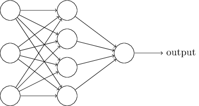
 input lines with an integration function
  . The total excitation computed in this way is then evaluated using an activation
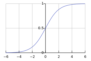
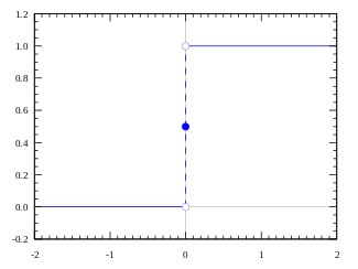
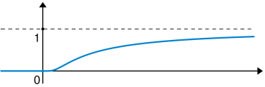
 . In perceptrons the integration function is the sum of the inputs. The activation (also called output function) compares the sum with a threshold. Later we will generalize
  to produce all values between 0 and 1. In the case of
  some functions other than addition can also be considered [454], [259]. In this case the networks can compute some difficult functions
 consisting of a set I of input sites, a set
  of output sites and a set
  of weighted directed edges. A directed edge is a tuple
  whereby
  ,
,  and
and  .
.

![python3 Python 3.2.3 (default, Mar 1 2013, 11:53:50) [GCC 4.6.3] on linux2 Type "help", "copyright", "credits" or "license" for more information. # 定義站站間『連接』事實 >>> from pyDatalog import pyDatalog >>> pyDatalog.create_terms('連接, 鄰近, 能達, 所有路徑') >>> +連接('台北車站', '中山') >>> +連接('台北車站', '善導寺') >>> +連接('台北車站', '西門') >>> +連接('台北車站', '台大醫院') >>> +連接('西門', '龍山寺') >>> +連接('西門', '小南門') >>> +連接('西門', '北門') >>> +連接('中山', '北門') >>> +連接('中山', '雙連') >>> +連接('中山', '松江南京') >>> +連接('中正紀念堂', '小南門') >>> +連接('中正紀念堂', '台大醫院') >>> +連接('中正紀念堂', '東門') >>> +連接('中正紀念堂', '古亭') >>> +連接('東門', '古亭') >>> +連接('東門', '忠孝新生') >>> +連接('東門', '大安森林公園') >>> +連接('善導寺', '忠孝新生') >>> +連接('松江南京', '忠孝新生') >>> +連接('忠孝復興', '忠孝新生') >>> +連接('松江南京', '行天宮') >>> +連接('松江南京', '南京復興') >>> +連接('中山國中', '南京復興') >>> +連接('台北小巨蛋', '南京復興') >>> +連接('忠孝復興', '南京復興') >>> +連接('忠孝復興', '忠孝敦化') >>> +連接('忠孝復興', '大安') >>> +連接('大安森林公園', '大安') >>> +連接('科技大樓', '大安') >>> +連接('信義安和', '大安') >>> +連接('信義安和', '世貿台北101') >>> </pre> 此處『連接』次序是『隨興』輸入的,一因『網路圖』沒有個經典次序,次因『事實』『陳述』不會因次序而改變,再 因『程序』上『pyDatalog』對此『事實』『次序』也並不要求。由於『連接』之次序有『起止』方向性,上面的陳述並不能代表那個『捷運網』,這可以 從下面程式片段得知。【<span style="color: #808080;">※ 在 pyDatalog 中,沒有變元的『查詢』 ask or query ,以輸出『set([()]) 』表示一個存在的事實,以輸出『None』表達所查詢的不是個事實。</span>】 <pre class="lang:sh decode:true"># 單向性 >>> pyDatalog.ask("連接('信義安和', '世貿台北101')") == set([()]) True >>> pyDatalog.ask("連接('世貿台北101', '信義安和')") == set([()]) False >>> pyDatalog.ask("連接('世貿台北101', '信義安和')") == None True >>> </pre> 所以我們必須給定『連接( □, ○)』是具有『雙向性』的,也就是 <span style="color: #ff9900;">連接<span class="crayon-sy">(</span><span class="crayon-i">X</span>站名<span class="crayon-sy">,</span><span class="crayon-i">Y</span>站名<span class="crayon-sy">)</span><span class="crayon-o"><=</span>連接<span class="crayon-sy">(</span><span class="crayon-i">Y</span>站名<span class="crayon-sy">,</span><span class="crayon-i">X</span>站名<span class="crayon-sy">)</span></span> ,這樣的『規則』 Rule 。由於 pyDatalog 的『語詞』 Term 使用前都必須『宣告』,而且『變元』必須『大寫開頭』,因此我們得用 <span style="color: #ff9900;">pyDatalog.create_terms('X站名, Y站名, Z站名, P路徑甲, P路徑乙')</span> 這樣的『陳述句』 Statement。【<span style="color: #808080;">※ 中文沒有大小寫,也許全部被當成了小寫,所以變元不得不以英文大寫起頭。</span>】 ─── 摘自《<a href="http://www.freesandal.org/?p=37256">勇闖新世界︰ 《 pyDatalog 》 導引《七》</a>》 <span style="color: #666699;">假使細思](http://www.freesandal.org/wp-content/ql-cache/quicklatex.com-f6d2dbbf270540e1b076e54dab9f778c_l3.png "Rendered by QuickLaTeX.com") z_j = \sum_i w_{ji} \cdot x_i + b_j$ 表達式,或許自可發現『 S 神經元』網絡計算與『矩陣』數學密切關聯︰
z_j = \sum_i w_{ji} \cdot x_i + b_j$ 表達式,或許自可發現『 S 神經元』網絡計算與『矩陣』數學密切關聯︰


 with multiplication as composition is


 就是
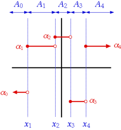
就是  的『鄰域』 neighborhood,而
  也就是
也就是  的『鄰域』 。所以函數上『一點』的連續性是說『這個點』的所有『指定鄰域』,都有一個『實數區間』──
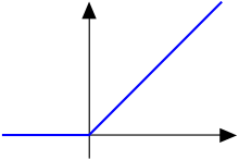
 時,『斜率』是
  ,在
,在  時,『斜率』為
  時『斜率』不存在!這使得我們必須研究一個函數在『每個點』之『鄰域』情況,於是數學步入了『解析的』 Analytic 時代。所謂『解析的』一詞是指『這類函數』在
  的『鄰域』,可以用『
 類函數。舉例來說
 類,而不是屬於
  類。
類。 類,但是它可以不是『解析函數』,比方說
 時無法用『泰勒級數』來作展開,因此不是『解析的』。

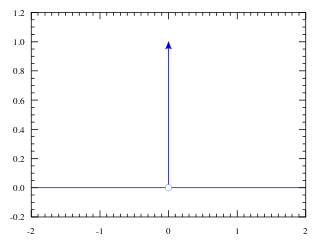
 ,而且這個『狄拉克
  函數』 Dirac Delta function 是這樣定義的


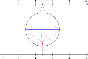
 的『擴張』一樣,他將『實數系』增入了『無窮小』 infinitesimals 元素
  ,魯濱遜創造出『超實數』 hyperreals
  ,形成了『超實數系』
  。那這個『無窮小』是什麼樣的『數』呢?對於『正無窮小』來說,任何給定的『正數』都比要它大,就『負無窮小』來講,它大於任何給定的『負數』。 『零』也就自然的被看成『實數系』裡的『無窮小』的了。假使我們說兩個超實數
  是『無限的鄰近』 indefinitly close,記作
  是指
是指  是個『無窮小』量。在這個觀點下,『無窮小』量不滿足『實數』的『阿基米德性質』。也就是說,對於任意給定的
  來講,
來講,  為『無窮小』量;而
  是『無限大』量。然而在『系統』與『自然』的『擴張』下,『超實數』的『算術』符合所有一般『代數法則』。
 與『虛部』
與『虛部』  取值『運算』一樣,『超實數』也有一個取值『運算』叫做『標準部份函數』Standard part function

 在
在  ,可以得到
,可以得到 
 ,那麼
,那麼 ![\frac{dy}{dx} = st \left[ \frac{\Delta y}{\Delta x} \right] = st \left[ \frac{(x + \Delta x)^2 - x^2}{\Delta x} \right]](http://www.freesandal.org/wp-content/ql-cache/quicklatex.com-027fed5e87d650562988caa58b710daf_l3.png "Rendered by QuickLaTeX.com")
![= st \left[2 x + \Delta x \right] = 2 x](http://www.freesandal.org/wp-content/ql-cache/quicklatex.com-9a657c7a5cc4ebefa63af6605c7ae82e_l3.png "Rendered by QuickLaTeX.com")


 。
。
