時間序列︰生成函數‧漸近展開︰當白努利遇上傅立葉《IV》

2017-04-20 懸鉤子

如果 $n$ 是巨量 $H \approx \infty$ ， $\therefore \frac{1}{k^{2H}}, \frac{1}{k^{2H+1}} \approx 0$ 。此時白努利多項式的傅立葉級數

$B_{2n} (x) = {(-1)}^{n+1} \frac{2 (2n)!}{{(2 \pi )}^{2n}} \sum \limits_{k=1}^{\infty} \frac{\cos(2 \pi k \cdot x)}{k^{2n}}$ ，

$B_{2n+1} (x) = {(-1)}^{n+1} \frac{2 (2n+1)!}{{(2 \pi )}^{2n+1}} \sum \limits_{k=1}^{\infty} \frac{\sin(2 \pi k \cdot x)}{k^{2n+1}}$ 。

只剩 $k=1$ 單項主導，趨近於

$B_{2H} (x) \approx {(-1)}^{H+1} \frac{2 (2H)!}{{(2 \pi )}^{2H}} \cos(2 \pi \cdot x)$ ，

$B_{2H+1} (x) \approx {(-1)}^{H+1} \frac{2 (2H+1)!}{{(2 \pi )}^{2H+1}} \sin (2 \pi \cdot x)$ 。

故於 $[0,1]$ 閉區間裡

$B_{2H} (x) = 0, \ x = \frac{1}{4} , \frac{3}{4}$ ，

$B_{2H+1} (x) = 0, \ x = 0 , \frac{1}{2} , 1$ 。

這時回顧先前『根』之考察︰

且讓我們嘗試運用此法更精細定位偶次 $2n$ 類在閉區間 $[0, 1]$ 之根 $B_{2n} (x) = 0$ 吧。此處重複使用

◎ 乘法公式

$m^{1-n} \cdot B_n (m \cdot x) = \sum \limits_{k=0}^{m-1} B_n (x + \frac{k}{m} ), \ m \ge 1$ 。

◎ 對稱公式

$B_n (1-x) = {(-1)}^n B_n (x), \ n \ge 0$ 。

簡單運算可得︰

△ $B_{2n} (\frac{1}{2}) = (2^{1-2n} -1) B_{2n}$

$B_{2n} (\frac{1}{2}) + B_{2n} (\frac{1}{2} + \frac{1}{2}) = 2^{1-2n} \cdot B_{2n} (2 \cdot \frac{1}{2})$

$B_{2n} (1) = B_{2n} (0) = B_{2n}$

△ $B_{2n} (\frac{1}{4}) = B_{2n} (\frac{3}{4}) = 2^{-2n} B_{2n} (\frac{1}{2}) = 2^{-2n} (2^{1-2n} -1) B_{2n}$

$B_{2n} (\frac{1}{4}) + B_{2n} (\frac{1}{4} + \frac{1}{2}) = 2^{1-2n} \cdot B_{2n} (2 \cdot \frac{1}{4})$

$B_{2n} (\frac{1}{4}) = B_{2n}(\frac{3}{4})$

△ $B_{2n} (\frac{1}{3}) = B_{2n} (\frac{2}{3}) = 2^{-1} (3^{1-2n} - 1) B_{2n}$

$B_{2n} (\frac{1}{3}) + B_{2n} (\frac{1}{3} + \frac{1}{3}) + B_{2n} (\frac{1}{3} + \frac{2}{3}) = 3^{1-2n} \cdot B_{2n} (3 \cdot \frac{1}{3})$

$B_{2n} (\frac{1}{3}) = B_{2n} (\frac{2}{3})$

△ $B_{2n} (\frac{1}{6}) = B_{2n} (\frac{5}{6}) = (2^{1-2n} -1)(3^{1-2n} -1) \frac{B_{2n}}{2}$

$B_{2n} (\frac{1}{6}) + B_{2n} (\frac{1}{6} + \frac{1}{2}) = 2^{1-2n} \cdot B_{2n} ( 2 \cdot \frac{1}{6})$

$B_{2n} (\frac{1}{6}) = (2^{1-2n} -1) B_{2n} (\frac{1}{3})$

因此可以歸結的說︰當 $n \ge 1$ 時， $B_{2n} (\frac{1}{2})$ 以及 $B_{2n} (\frac{1}{3})$ 、 $B_{2n} (\frac{1}{4})$ 與 $B_{2n}$ 異號。然而 $B_{2n} (\frac{1}{6})$ 和 $B_{2n}$ 同號。故知 $B_{2n} = 0$ 有一根 $r$ 落在 $(\frac{1}{6}, \frac{1}4})$ 開區間中。因著『偶對稱性』的要求，另一根定然是 $1 - r$ ，且知其落於 $(\frac{3}{4}, \frac{5}{6})$ 開區間也☆☆

─── 摘自《時間序列︰生成函數‧漸近展開︰白努利多項式之根《六》》

暗示著 $r_{2n}$ 將越來越大，當 $n \to \infty$ 時， $r_{2n} \to \frac{1}{4}$ 了。可借著數值計算驗證如下︰

pi@raspberrypi:~ \frac{1}{4} - \frac{1}{\pi \cdot 2^{2n}} < r_{2n} < r_{2(n+1)} < \frac{1}{4}, \ n \ge 1B_{2m} ( \frac{1}{4} ) \cdot B_{2m} < 0, m \ge 1B_{2(n+1)} (r_{2n}) \cdot B_{2(n+1)} > 0r_{2n} < r_{2(n+1)}1 < \zeta({2n}) = \sum \limits_{k=1}^{\infty} \frac{1}{k^{2n}} \le 1 + \frac{2n+1}{2n-1} \cdot \frac{1}{2^{2n}} \le 1 + \frac{3}{2^{2n}} \le 1 + \frac{3}{4} < 2\sum \limits_{k=3}^{\infty} \frac{1}{k^{2n}} \le \sum \limits_{k=3}^{\infty}  \int_{k-1}^{k} \frac{dt}{t^{2n}} = \int_{2}^{\infty} \frac{dt}{t^{2n}} = \frac{2}{2n - 1} \cdot \frac{1}{2^{2n}}1 < \sum \limits_{k=1}^{\infty} \frac{1}{k^{2n}} \le 1 + \frac{1}{2^{2n}} + \frac{2}{2n-1} \cdot \frac{1}{2^{2n}} = 1 + \frac{2n+1}{2n-1} \frac{1}{2^{2n}}\lim \limits_{n \to \infty} \sum \limits_{k=1}^{\infty} \frac{1}{k^{2n}}  = 1n \ge 1, 4n - 4 \ge 0, 3(2n-1) - (2n+1) = 4n-4 \ge 01 < \sum \limits_{k=1}^{\infty} \frac{1}{k^{2n}} \le 1+ 3 \cdot \frac{1}{2^2} = 1 + \frac{3}{4}\sin(x) \le x, \ x \ge0\lim \limits_{x \to 0} \frac{\sin(x)}{x} = 1\triangle OBB^{'}\sphericalangle OBB^{'}\Box OBCB^{'}\sin{\theta} \cos{\theta} < \theta < \tan{\theta}\cos{\theta} < \frac{ \theta}{\sin{\theta} } < \frac{1}{\cos{\theta}}\sphericalangle OBB^{'}\triangle OBB^{'}\therefore x > \sin (x), \ x>0\cos (x) > 1 - \frac{x^2}{2}, \ x > 0f(x) = \cos(x) - \left( 1 - \frac{x^2}{2} \right)f(0) = 0f^{'} (x) = - \sin (x) + x > 0, \ x >0f (x)\sin (x) > x - \frac{x^3}{6}, \ x > 0B_{2n} (\frac{1}{4} - \frac{1}{\pi \cdot 2^{2n}} ) \cdot B_{2n} B_{2(n+2)} (r_{2n} ) \cdot B_{2(n+1)} $
之『正負號』為『正』，應留與善學好思之讀者的吧☆

樹莓派、樹莓派之學習、樹莓派之教育

時間序列︰生成函數‧漸近展開︰當白努利遇上傅立葉《III》

2017-04-19 懸鉤子

諺語說：人有失手，馬有亂蹄，這件事難保不會出紕漏。簡單的講︰吃燒餅哪有不掉芝麻的。是說不是『不可能』的，也就是『可能』的！那麼『百分之百』之『可能性』是否就意味『必然』的哩？科學家費米以擅長『合理估算』著名，他講『大象說』如雷貫耳，那麼當他提出

費米悖論

費米悖論（Fermi paradox，又稱費米謬論）闡述的是對地外文明存在性的過高估計和缺少相關證據之間的矛盾^[1]。宇宙驚人的年齡和龐大的星體數量意味著，除非地球是一個特殊的例子，否則地外生命應該廣泛存在^[2] 。在1950年的一次非正式討論中，物理學家恩里科·費米問道，如果銀河系存在大量先進的地外文明，那麼為什麼連飛船或者探測器之類的證據都看不到。對這個話題更加具體的探討最早出現在1975年麥克·哈特的文章中，有時也被叫做麥克·哈特悖論^[3]。另一個緊密相關的問題是大沉默——即使難以星際旅行，如果生命是普遍存在的話，為什麼我們探測不到電磁信號？有人嘗試通過尋找地外文明的證據來解決費米悖論，也提出這些生命可能不具備人類的智慧。也有學者認為高等地外文明根本不存在，或者非常稀少以至於人類不可能聯繫得上。地球殊異假說有時被認為為費米悖論提供了一種解釋的答案。

從哈特開始，很多人開始發展關於地外文明的科學理論或模型。大部分工作都引用費米悖論作為參考。很多相關的問題已經得到重視，內容包括天文學、生物學、生態學和哲學。新興的天體生物學給問題的解決引入了跨學科的研究手段。

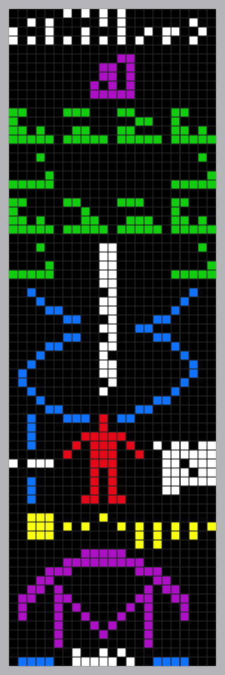
阿雷西博信息，顏色是用作分類，信息本身沒有任何顏色。人類首次嘗試利用電磁波尋找外星生命

時，豈可掉以輕心乎？尤其是它還關切人類在宇宙之地位耶？？

悖論基礎

費米悖論講述的是有關尺度和機率的論點和稀缺的證據之間的矛盾，其基本內涵表述如下：

宇宙顯著的尺度和年齡意味著高等地外文明應該存在。
The apparent size and age of the universe suggest that many technologically advanced extraterrestrial civilizations ought to exist.
但是，這個假設得不到充分的證據支持。
However, this hypothesis seems inconsistent with the lack of observational evidence to support it.

費米悖論的第一點，即尺度問題，是一個數量級估計：銀河系大約有2500億（2.5 x 10¹¹）顆恆星，可觀測宇宙內則有700垓（7 x 10²²）顆。即使智慧生命以很小的機率出現在圍繞這些恆星的行星中，那麼僅僅在銀河系內就應該有相當大數量的文明存在。這也符合平庸原理的觀點，即地球不是特殊的，僅僅是一個典型的行星，具有和其他星體相同的規律和現象。有人用德雷克公式來支持這個論點，儘管這個式子的基礎正在受到質疑。

費米悖論的第二點是對尺度觀點的答覆：考慮到智慧生命克服資源稀缺的能力和對外擴張的傾向性，任何高等文明都很可能會尋找新的資源和開拓他們所在的恆星系統，然後是涉足鄰近的星系。因為在宇宙誕生137億年之後，我們沒有在地球或可觀測宇宙的其他地方，找到其他智慧生命存在的切實可靠的證據；可以認為智慧生命是很稀少的，或者說我們對智慧生命的一般行為的理解是有誤的。

費米悖論可以表述成兩種形式。一種是「為什麼沒有發現外星人或者外星物品？」如果星際旅行是可行的話，即使是用人類造的飛船這樣緩慢地旅行，也只需要5百萬到5千萬年去征服星系。就算不考慮宇宙尺度，在地質學尺度上這也是一個相當短的時間。因為有很多年齡比太陽更大的恆星，或者因為智慧生命可能進化得更早，這個問題就變成為什麼星系還沒有被殖民。即使殖民對所有外星文明來說是不合實際的或者是不想去做的，大規模的星際探索也應該是有可能（探索的方式和理論上的探測器會在下文具體討論）。然而，沒有任何關於殖民和探索的證據得到承認。

上面的討論可能並沒有把宇宙作為整體考慮在內，因為星際旅行的次數問題就足以解釋為什麼地球上缺少外星生物的證據。但是，問題就變成「為什麼我們看不到智慧生命的跡象？」，因為足夠高等的文明應該能在可觀測宇宙的較大範圍內被看見。即使這些文明是很稀少的，尺度問題的討論暗示他們可能在宇宙歷史中的某一段存在過。因為他們在相當長的一段時間內能夠被觀測到，我們視野範圍內應該能找到很多他們起源地的跡象。然而，沒有任何確切的地外文明的觀測證據。

相同的，以尺度和機率的角度與視野來觀察，地球屬於適居帶的行星，擁有且滿足一切生物物種維持生命、生存和演化的所有條件，然而事實上從地球歷史中的顯生宙開始至今，在這長達五億多年的歲月間和數百萬的生物物種中，只有一個物種成功的演化成為高等智慧生命－「人類」，而非多種多元的高等智慧生物並存於地球上，這顯示了在「相同條件」下，「高等智慧生命」並非如此的輕易出現和存在。同地球殊異假說一般，這或許為費米悖論提供了其中一個答案。

故早已實至名歸矣！

名字起源

1950年，物理學家恩里科·費米在洛斯阿拉莫斯國家實驗室工作。他在一次去吃午飯的路上，和同事埃米爾·康佩斯基、愛德華·泰勒、赫伯特·約克有一段普通的交談^[4]。一開始，他們談論當時流行的UFO報導和阿蘭·鄧的漫畫^[5]。漫畫把市內垃圾箱的失蹤歸咎於外星人的掠奪。接著他們談到未來十年內，人類能夠觀測到超光速運動的物體的機率大小。泰勒認為是百萬分之一，但費米覺得接近於十分之一。然後話題又轉向其他方面，直到午餐時費米突然問道「Where are they？」，即「他們在哪裡？」（也有說法是「Where is everybody?」，即「其他人在哪裡」)^[6]。據其中一個在場人士回憶，費米當時用了幾個估計的數值做了一系列的快速計算。（費米很擅長於用基本原理和少量的數據做出數量估計，詳見費米問題）依靠估算，他當時的結論是地球應該在很早以前被外星人訪問過，而且被訪問的次數遠不止一次^[6]^[4]。

其後有人用『模態邏輯』

Modal logic

Modal logic is a type of formal logic primarily developed in the 1960s that extends classical propositional and predicate logic to include operators expressing modality. A modal—a word that expresses a modality—qualifies a statement. For example, the statement “John is happy” might be qualified by saying that John is usually happy, in which case the term “usually” is functioning as a modal. The traditional alethic modalities, or modalities of truth, include possibility (“Possibly, p“, “It is possible that p“), necessity (“Necessarily, p“, “It is necessary that p“), and impossibility (“Impossibly, p“, “It is impossible that p“).^[1] Other modalities that have been formalized in modal logic include temporal modalities, or modalities of time (notably, “It was the case that p“, “It has always been that p“, “It will be that p“, “It will always be that p“),^[2]^[3] deontic modalities (notably, “It is obligatory that p“, and “It is permissible that p“), epistemic modalities, or modalities of knowledge (“It is known that p“)^[4] and doxastic modalities, or modalities of belief (“It is believed that p“).^[5]

A formal modal logic represents modalities using modal operators. For example, “It might rain today” and “It is possible that rain will fall today” both contain the notion of possibility. In a modal logic this is represented as an operator, “Possibly”, attached to the sentence “It will rain today”.

The basic unary (1-place) modal operators are usually written “□” for “Necessarily” and “◇” for “Possibly”. In a classical modal logic, each can be expressed by the other with negation:

\Diamond P\leftrightarrow \lnot \Box \lnot P;

\Box P\leftrightarrow \lnot \Diamond \lnot P.

Thus it is possible that it will rain today if and only if it is not necessary that it will not rain today; and it is necessary that it will rain today if and only if it is not possible that it will not rain today. Alternative symbols used for the modal operators are “L” for “Necessarily” and “M” for “Possibly”.^[6]

解析『語義』，發現『機率』的『不可能』性其實不同於『必然』之『不可能』，是否解決了『問題』的呢？？？假使將桌上之一塊木片，以其桌邊為坐標系，然後去此木片裡的所有有理數點，請問這時它的面積如何計算哩！！！

勒貝格測度

數學上，勒貝格測度是賦予歐幾里得空間的子集一個長度、面積、或者體積的標準方法。它廣泛應用於實分析，特別是用於定義勒貝格積分。可以賦予一個體積的集合被稱為勒貝格可測；勒貝格可測集A的體積或者說測度記作λ(A)。一個值為∞的勒貝格測度是可能的，但是即使如此，在假設選擇公理成立時，Rⁿ的所有子集也不都是勒貝格可測的。不可測集的「奇特」行為導致了巴拿赫-塔斯基悖論這樣的命題，它是選擇公理的一個結果。

問題起源

人們知道，區間的長度可以定義為端點值之差。若干個不交區間的並的長度應當是它們的長度之和。於是人們希望將長度的概念推廣為比區間更複雜的集合。

我們想構造一個映射m，它能將實數集的子集E映射為非負實數mE 。稱這樣的映射（集函數）為集合E的測度。最理想的情況應該是m具有以下性質：

mE對於實數集的所有子集E都有定義。
對於一個區間I，mI應當等於其長度（端點數值之差）。
如果{E_n}是一列不相交的集合，並且m在其上有定義，那麼 $m(\cup E_n) = \sum mE_n$ 。
m具有平移不變性，即如果一個m有定義的集合E的每個元素都加一個相同的實數（定義為 $\{x + y | x \in E\}$ ，記作E+y），那麼m(E+y)=mE。

遺憾的是，這樣的映射（集函數）是不存在的。人們只能退而求其次，尋找滿足其中部分條件的映射。其中一個例子是若爾當測度，它只滿足有限可加性（第三條性質希望具有可數可加性）。勒貝格測度是滿足後三條性質的例子。

依舊祇是『語義』的『解釋』吧？△

零測集

主條目：零測集

Rⁿ的子集是零測集，如果對於每一個ε > 0，它都可以用可數個區間的乘積來覆蓋，其總體積最多為ε。所有可數集都是零測集。

如果Rⁿ的子集的豪斯多夫維數小於n，那麼它就是關於n維勒貝格測度的零測集。在這裡，豪斯多夫維數是相對於Rⁿ上的歐幾里得度量（或任何與其等價的利普希茨度量）。另一方面，一個集合可能拓撲維數小於n，但具有正的n維勒貝格測度。一個例子是史密斯-沃爾泰拉-康托爾集，它的拓撲維數為0，但1維勒貝格測度為正數。

為了證明某個給定的集合A是勒貝格可測的，我們通常嘗試尋找一個「較好」的集合B，與A只相差一個零測集，然後證明B可以用開集或閉集的可數交集和並集生成。

誰又可壟斷『意義』之『詮釋』啊！▼

所以許多事會發生『同義反復』之『現象』，或知或不知而已夫。科學終究建立於『觀察』與『實驗』也☆☆

因此聽聞︰

方法能傳精神難，善用方法不簡單。

天生精神自己有，博學廣思勤鍛鍊。

Kline 教授說︰

$s_{2n} = \sum \limits_{\nu=1}^{\infty} \frac{1}{{\nu}^{2 n}} = {(-1)}^{n-1} \frac{{(2 \pi)}^{2 n}}{2 (2n)!} B_{2 n}$

此處 $B_{2n}$ 為白努利數。

是歐拉最好的勝利。

─ 摘自《時間序列︰生成函數‧漸近展開︰白努利 □○《九下》》

且又及於︰

為什麼以 $d_{4k}$ 為中心立論呢？答案請參考上一篇。這裡只強調有值也。

$B_{4n} = - \frac{2(4n)!}{(2 \pi)^{4n}} \sum \limits_{\nu=1}^{\infty} \frac{1}{{\nu}^{4 n}}$ 。
※

$\sum \limits_{k=3}^{\infty} \frac{1}{k^{4n}} \le \sum \limits_{k=3}^{\infty} \int_{k-1}^{k} \frac{dt}{t^{4n}} = \int_{2}^{\infty} \frac{dt}{t^{4n}} = \frac{2}{4n - 1} \cdot \frac{1}{2^{4n}}$

$1 < \sum \limits_{k=1}^{\infty} \frac{1}{k^{4n}} \le 1 + \frac{1}{2^{4n}} + \frac{2}{4n-1} \cdot \frac{1}{2^{4n}} = 1 + \frac{4n+1}{4n-1} \frac{1}{2^{4n}}$

$\lim \limits_{n \to \infty} \sum \limits_{k=1}^{\infty} \frac{1}{k^{4n}} = 1$ 。

而且 $n \ge 1, 4n - 3 \ge 0, 2(4n-1) - (4n+1) = 4n-3 \ge 0$ ，所以

$1 < \sum \limits_{k=1}^{\infty} \frac{1}{k^{4n}} \le 1+ 2 \cdot \frac{1}{2^4} = 1 + \frac{1}{8}$ 。

─── 摘自《時間序列︰生成函數‧漸近展開︰白努利多項式之根《八》》

或將會『揣想』和『衡量』

$\frac{B_{2n+2}}{B_{2n}} = \frac {\frac{2 (2n+2)!}{{(2 \pi)}^{2n+2}}}{\frac{2 (2n)!}{{(2 \pi)}^{2n}}} = \frac{(2n+2)(2n+1)}{4 {\pi}^2}$ 焉？

認為

$B_n (x) = B_0 x^n + \binom{n}{1} B_1 x^{n-1} + \cdots + \binom{n}{n-1} B_{n-1} x^1 + B_n = 0, \ B_0 = 1$

$= x^n ( 1 + \binom{n}{1} \frac{B_1}{x} + \cdots + \binom{n}{n-1} \frac{B_{n-1}}{x^{n-1}}) + B_n = 0$

，當 $n$ 很大，而且 $x$ 足夠大 $\binom{n}1} \frac{B_1}{x} + \cdots + \binom{n}{n-1} \frac{B_{n-1}}{x^{n-1}} \approx 0$ 時，難道不是

$\approx x^n + B_n = 0$ 耶？ $\therefore x \approx \sqrt[n]{-B_n}$ 。

那麼當 $n = 2k+1, \ k \ge 1$ 是奇數， $B_n =0$ ，因此 $x=0$ 合理乎？若是 $- B_n <0$ ，彷彿 $n=4k+2$ 的情況， $x$ 將為虛數耶？？故而偏好 $n=4k$ 之形式嗎？☆

如果真如是，所謂『邏輯一致性』或『意義自恰性』將迫使

$\frac{B_{4k+1}}{x} = x^{4k} (1+ \binom{4k+1}{1} \frac{B_1}{x} + \cdots + \binom{4k+1}{4k-1} \frac{B_{4k-1}}{x^{4k-1}}) + \binom{4k+1}{4k} B_{4k} = 0$

不得不然矣！☆

故 $\therefore x \approx \sqrt[{4k}]{ -B_{4k}(4k+1)} \approx \sqrt[{4k}] {-B_{4k}}$ 哉◎◎

樹莓派、樹莓派之學習、樹莓派之教育

時間序列︰生成函數‧漸近展開︰當白努利遇上傅立葉《II》

2017-04-18 懸鉤子

數學之『進步』怎麼說勒？果是當一個『困難』的問題︰

『巴塞爾問題』是一個著名的『數論問題』，最早由『皮耶特羅‧門戈利』在一六四四年所提出。由於這個問題難倒了以前許多的數學家，因此一七三五年，當『歐拉』一解出這個問題後，他馬上就出名了，當時『歐拉』二十八歲。他把這個問題作了一番推廣，他的想法後來被『黎曼』在一八五九年的論文《論小於給定大數的質數個數》 On the Number of Primes Less Than a Given Magnitude中所採用，論文中定義了『黎曼ζ函數』，並證明了它的一些基本的性質。那麼為什麼今天稱之為『巴塞爾問題』的呢？因為『此處』這個『巴塞爾』，它正是『歐拉』和『伯努利』之家族的『家鄉』。那麼就這麽樣的一個『級數的和』 $\sum \limits_{n=1}^\infty \frac{1}{n^2} = \lim \limits_{n \to +\infty}\left(\frac{1}{1^2} + \frac{1}{2^2} + \cdots + \frac{1}{n^2}\right)$ 能有什麼『重要性』的嗎？即使僅依據『發散級數』 divergent series 的『可加性』 summable 之『歷史』而言，或又得再過了百年的時間之後，也許早已經是『柯西』之『極限觀』天下後『再議論』的了！！因是我們總該看看『歷史』上『歐拉』自己的『論證』的吧！！

巴塞爾問題
$\sum_{n=1}^{\infty}\frac{1}{n^2} = \frac{\pi^2}{6}$

邏輯之歐拉圖

假使說『三角函數』 $\sin{x}$ 可以表示為 $\sin(x) = x - \frac{x^3}{3!} + \frac{x^5}{5!} - \frac{x^7}{7!} + \cdots$ ，那麼『除以』 $x$ 後，將會得到 $\frac{\sin(x)}{x} = 1 - \frac{x^2}{3!} + \frac{x^4}{5!} - \frac{x^6}{7!} + \cdots$ ，然而 $\sin{x}$ 的『根』是 $x = n\cdot\pi$ ，由於『除以』 $x$ 之緣故，因此 $n \neq 0$ ，所以 $n = \pm1, \pm2, \pm3, \dots$ ，那麼 $\frac{\sin(x)}{x}$ 應該會『等於』 $\left(1 - \frac{x}{\pi}\right)\left(1 + \frac{x}{\pi}\right)\left(1 - \frac{x}{2\pi}\right)\left(1 + \frac{x}{2\pi}\right)\left(1 - \frac{x}{3\pi}\right)\left(1 + \frac{x}{3\pi}\right) \cdots$ ，於是也就『等於』 $\left(1 - \frac{x^2}{\pi^2}\right)\left(1 - \frac{x^2}{4\pi^2}\right)\left(1 - \frac{x^2}{9\pi^2}\right) \cdots$ ，若是按造『牛頓恆等式』，考慮 $x^2$ 項的『係數』，就會有 $- \left(\frac{1}{\pi^2} + \frac{1}{4\pi^2} + \frac{1}{9\pi^2} + \cdots \right) = -\frac{1}{\pi^2}\sum_{n=1}^{\infty}\frac{1}{n^2}$ ，然而 $\frac{\sin(x)}{x}$ 之『 $x^2$ 項』的『係數』是『 $- \frac{1}{3!} = -\frac{1}{6}$ 』，所以 $-\frac{1}{6} = -\frac{1}{\pi^2}\sum \limits_{n=1}^{\infty}\frac{1}{n^2}$ ，於是 $\sum \limits_{n=1}^{\infty}\frac{1}{n^2} = \frac{\pi^2}{6}$ 。那麼『歐拉』是『對』的嗎？還是他還是『錯』的呢？？

─── 摘自《【Sonic π】電聲學之電路學《四》之《 V!》‧下中》

而今可從 ${\tilde{B}}_{2n} (x) = {(-1)}^{n+1} \frac{2 (2n)!}{{(2 \pi )}^{2n}} \sum \limits_{k=1}^{\infty} \frac{\cos(2 \pi k \cdot x)}{k^{2n}}$ ，代入 $n=1$ ，得到

${\tilde{B}}_2 (x) = {(-1)}^{1+1} \frac{2 (2 \cdot 1)!}{{(2 \pi )}^{2 \cdot 1}} \sum \limits_{k=1}^{\infty} \frac{\cos(2 \pi k \cdot x)}{k^{2 \cdot 1}}$

$= \frac{1}{{\pi}^2} \sum \limits_{k=1}^{\infty} \frac{\cos(2 \pi k \cdot x)}{k^{2}}$ 。於是

${\tilde{B}}_2 (\frac{1}{2}) = B_2 (\frac{1}{2} = (x^2 - x + \frac{1}{6}) |_{x=\frac{1}{2}} = - \frac{1}{12}$

$= \frac{1}{{\pi}^2} \sum \limits_{k=1}^{\infty} \frac{ {(-1)}^{k} }{k^2}$

$= \frac{1}{{\pi}^2} \left[ - \sum \limits_{k=1}^{\infty} \frac{1}{ {(2k-1)}^2 } + \sum \limits_{k=1}^{\infty} \frac{1}{ {(2k)}^2 } \right]$

$= \frac{1}{{\pi}^2} \left[ - \frac{3}{4} \sum \limits_{k=1}^{\infty} \frac{1}{ {(k)}^2 } + \frac{1}{4} \sum \limits_{k=1}^{\infty} \frac{1}{ {(k)}^2 } \right]$

$= \frac{1}{{\pi}^2} \left[- \frac{1}{2} \sum \limits_{k=1}^{\infty} \frac{1}{ {(k)}^2 } \right]$

$= - \frac{1}{2 {\pi}^2} \frac{1}{2} \sum \limits_{k=1}^{\infty} \frac{1}{ {k}^2 }$ ，『容易』知道

$\sum \limits_{k=1}^{\infty} \frac{1}{ {k}^2 } = \frac{{\pi}^2}{6}$ 矣。

這樣就能說成『創新』了嗎？假使代入 $x=0$ ，可得『歐拉最好的勝利』
${\tilde{B}}_{2n} (0) = {(-1)}^{n+1} \frac{2 (2n)!}{{(2 \pi )}^{2n}} \sum \limits_{k=1}^{\infty} \frac{1}{k^{2n}}$

，更清楚表明之乎！！

不知誰知其後又將有

Riemann zeta function

The Riemann zeta function or Euler–Riemann zeta function, $ζ (s)$ , is a function of a complex variable s that analytically continues the sum of the Dirichlet series

\zeta (s)=\sum _{n=1}^{\infty }{\frac {1}{n^{s}}}

for when the real part of $s$ is greater than 1. More general representations of $ζ (s)$ for all $s$ are given below. The Riemann zeta function plays a pivotal role in analytic number theory and has applications in physics, probability theory, and applied statistics.

As a function of a real variable, Leonhard Euler first introduced and studied it in the first half of the eighteenth century without using complex analysis, which was not available at the time. Bernhard Riemann‘s 1859 article “On the Number of Primes Less Than a Given Magnitude” extended the Euler definition to a complex variable, proved its meromorphic continuation and functional equation, and established a relation between its zeros and the distribution of prime numbers.^[2]

The values of the Riemann zeta function at even positive integers were computed by Euler. The first of them, $ζ (2)$ , provides a solution to the Basel problem. In 1979 Apéry proved the irrationality of $ζ (3)$ . The values at negative integer points, also found by Euler, are rational numbers and play an important role in the theory of modular forms. Many generalizations of the Riemann zeta function, such as Dirichlet series, Dirichlet $L$ -functions and $L$ -functions, are known.

Definition

Bernhard Riemann’s article on the number of primes below a given magnitude.

The Riemann zeta function $ζ (s)$ is a function of a complex variable $s = σ + it$ . (The notation $s$ , $σ$ , and $t$ is used traditionally in the study of the zeta function, following Riemann.)

The following infinite series converges for all complex numbers $s$ with real part greater than 1, and defines $ζ (s)$ in this case:

\zeta (s)=\sum _{n=1}^{\infty }n^{-s}={\frac {1}{1^{s}}}+{\frac {1}{2^{s}}}+{\frac {1}{3^{s}}}+\cdots \qquad \sigma =\operatorname {Re} (s)>1.

It can also be defined by the integral

\zeta (s)={\frac {1}{\Gamma (s)}}\int _{0}^{\infty }{\frac {x^{s-1}}{e^{x}-1}}\mathrm {d} x

where $Γ(s)$ is the gamma function.

The Riemann zeta function is defined as the analytic continuation of the function defined for $σ > 1$ by the sum of the preceding series.

Leonhard Euler considered the above series in 1740 for positive integer values of $s$ , and later Chebyshev extended the definition to $Re(s) > 1$ .^[3]

The above series is a prototypical Dirichlet series that converges absolutely to an analytic function for $s$ such that $σ > 1$ and diverges for all other values of $s$ . Riemann showed that the function defined by the series on the half-plane of convergence can be continued analytically to all complex values $s \neq 1$ . For $s = 1$ the series is the harmonic series which diverges to $+\infty$ , and

\lim _{s\to 1}(s-1)\zeta (s)=1.

Thus the Riemann zeta function is a meromorphic function on the whole complex $s$ -plane, which is holomorphic everywhere except for a simple pole at $s = 1$ with residue 1.

！乃今人們常常談起

特殊函數

特殊函數是指一些具有特定性質的函數，一般有約定俗成的名稱和記號，例如伽瑪函數、貝索函數、菲涅耳積分等。它們在數學分析、泛函分析、物理研究、工程應用中有著舉足輕重的地位。許多特殊函數是微分方程的解或基本函數的積分，因此積分表中常常會出現特殊函數，特殊函數的定義中也經常會出現積分。傳統上對特殊函數的分析主要基於對其的數值展開基礎上。隨著電子計算的發展，這個領域內開創了新的研究方法。因為微分方程的對稱性在數學和物理中的重要性，特殊函數理論也與李群和李代數密切相關。

事實上，對於哪些函數屬於特殊函數，並沒有明確的規定。函數列表中列出了一些通常被認為的特殊函數。廣義上，基本超越函數（即指數函數、對數函數、非有理次冪的冪函數、雙曲函數、三角函數等周期函數）也稱為特殊函數。

的耶？？

樹莓派、樹莓派之學習、樹莓派之教育

時間序列︰生成函數‧漸近展開︰當白努利遇上傅立葉《I》

2017-04-17 懸鉤子

如何求取白努利多項式周期函數 ${\tilde {B}}_{n} (x) = B_n (x - \lfloor x \rfloor)$ 之傅立葉級數呢？

傅立葉級數

在數學中，傅立葉級數（Fourier series, /ˈfɔərieɪ/）是把類似波的函數表示成簡單正弦波的方式。更正式地說，它能將任何周期函數或周期訊號分解成一個（可能由無窮個元素組成的）簡單振盪函數的集合，即正弦函數和餘弦函數（或者，等價地使用複指數）。離散時間傅立葉轉換是一個周期函數，通常用定義傅立葉級數的項進行定義。另一個應用的例子是Z轉換，將傅立葉級數簡化為特殊情形 |z|=1。傅立葉級數也是取樣定理原始證明的核心。傅立葉級數的研究是傅立葉分析的一個分支。

歷史

傅立葉級數得名於法國數學家約瑟夫·傅立葉(1768年–1830年)，他提出任何函數都可以展開為三角級數。此前數學家如拉格朗日等已經找到了一些非周期函數的三角級數展開，而認定一個函數有三角級數展開之後，通過積分方法計算其係數的公式，歐拉、達朗貝爾和克萊羅早已發現，傅立葉的工作得到了丹尼爾·伯努利的贊助^[1]。傅立葉介入三角級數用來解熱傳導方程，其最初論文在1807年經拉格朗日、拉普拉斯和勒讓德評審後被拒絕出版，他的現在被稱為傅里葉逆轉定理的理論後來發表於1820年的《熱的解析理論》中。將周期函數分解為簡單振盪函數的總和的最早想法，可以追溯至公元前3世紀古代天文學家的均輪和本輪學說。

傅立葉級數在數論、組合數學、訊號處理、機率論、統計學、密碼學、聲學、光學等領域都有著廣泛的應用。

定義

在這一節中，s(x) 表示實變量 x 的一個函數，且 s 在 [x₀, x₀ + P] 上可積，x₀ 和 P 為實數。我們將嘗試用諧波關係的正弦函數的無窮和或級數來表示該區間內的 s 。在區間外，級數以 P 為周期（頻率為 1/P）。若 s 也具有該性質，則它的近似在整個實數線上有效。我們可以從有限求和（或部分和）開始：

</span

$s_{N}(x)$ 為周期為 P 的周期函數。運用恆等式：

</span

</span

函數 s(x) （紅色）是六個不同幅度的諧波關係的正弦函數的和。它們的和叫做傅立葉級數。傅立葉轉換 S(f) （藍色），針對幅度與頻率進行描繪，顯示出6種頻率和它們的幅度。

我們還可以用這些等價形式書寫這個函數：

${\begin{aligned}s_{N}(x)&={\frac {a_{0}}{2}}+\sum _{{n=1}}^{N}\left(\overbrace {a_{n}}^{{A_{n}\sin(\phi _{n})}}\cos({\tfrac {2\pi nx}{P}})+\overbrace {b_{n}}^{{A_{n}\cos(\phi _{n})}}\sin({\tfrac {2\pi nx}{P}})\right)\\&=\sum _{{n=-N}}^{N}c_{n}\cdot e^{{i{\tfrac {2\pi nx}{P}}}},\end{aligned}}$

其中：

c_{n}\ {\stackrel {{\mathrm {def}}}{=}}\ {\begin{cases}{\frac {A_{n}}{2i}}e^{{i\phi _{n}}}={\frac {1}{2}}(a_{n}-ib_{n})&{\text{for }}n>0\\{\frac {1}{2}}a_{0}&{\text{for }}n=0\\c_{{|n|}}^{*}&{\text{for }}n<0.\end{cases}}

當係數（即傅立葉係數）以下面方式計算時：^[2]

a_{n}={\frac {2}{P}}\int _{{x_{0}}}^{{x_{0}+P}}s(x)\cdot \cos({\tfrac {2\pi nx}{P}})\ dx

b_{n}={\frac {2}{P}}\int _{{x_{0}}}^{{x_{0}+P}}s(x)\cdot \sin({\tfrac {2\pi nx}{P}})\ dx

c_{n}={\frac {1}{P}}\int _{{x_{0}}}^{{x_{0}+P}}s(x)\cdot e^{{-i{\tfrac {2\pi nx}{P}}}}\ dx,

$s_{N}(x)$ 在 $[x_{0},\ x_{0}+P]$ 近似了 $s(x)$ ，該近似程度會隨著 N → ∞ 逐漸改善。這個無窮和 $s_{{\infty }}(x)$ 叫做 $s$ 的傅立葉級數表示。在工程應用中，一般假定傅立葉級數除了在不連續點以外處處收斂，原因是工程上遇到的函數比數學家提供的這個假定的反例表現更加良好。特別地，傅立葉級數絕對收斂且均勻收斂於 s(x)，只要在 s(x) 的導數（或許不會處處存在）是平方可積的。^[3] 如果一個函數在區間 [x₀, x₀+P]上是平方可積的，那麼此傅立葉級數在幾乎所有點都收斂於該函數。傅立葉級數的收斂性取決於函數有限數量的極大值和極小值，這就是通常稱為傅立葉級數的狄利克雷條件。參見傅立葉級數的收斂性之一。對於廣義函數或分布也可以用範數或弱收斂定義傅立葉係數.

且讓我們介紹數學分析裡常用之技巧『分部積分法』︰

Integration by parts

In calculus, and more generally in mathematical analysis, integration by parts or partial integration is a theorem that relates the integral of a product of functions to the integral of their derivative and antiderivative. It is frequently used to transform the antiderivative of a product of functions into an antiderivative for which a solution can be more easily found. The rule can be derived in one line simply by integrating the product rule of differentiation.

If $u$ = $u (x)$ and $du$ = $u'(x) dx$ , while $v$ = $v (x)$ and $dv$ = $v'(x) dx$ , then integration by parts states that:

{\begin{aligned}\int _{a}^{b}u(x)v'(x)\,dx&=[u(x)v(x)]_{a}^{b}-\int _{a}^{b}u'(x)v(x)dx\\&=u(b)v(b)-u(a)v(a)-\int _{a}^{b}u'(x)v(x)\,dx\end{aligned}}

or more compactly:

\int u\,dv=uv-\int v\,du.\!

More general formulations of integration by parts exist for the Riemann–Stieltjes and Lebesgue–Stieltjes integrals. The discrete analogue for sequences is called summation by parts.

Visualization

Graphical interpretation of the theorem. The pictured curve is parametrized by the variable t.

Define a parametric curve by (x, y) = (f(t), g(t)). Assuming that the curve is locally one-to-one, we can define

x(y)=f(g^{-1}(y))

y(x)=g(f^{-1}(x))

The area of the blue region is

A_{1}=\int _{y_{1}}^{y_{2}}x(y)dy

Similarly, the area of the red region is

A_{2}=\int _{x_{1}}^{x_{2}}y(x)dx

The total area A₁ + A₂ is equal to the area of the bigger rectangle, x₂y₂, minus the area of the smaller one, x₁y₁:

\overbrace {\int _{y_{1}}^{y_{2}}x(y)dy} ^{A_{1}}+\overbrace {\int _{x_{1}}^{x_{2}}y(x)dx} ^{A_{2}}={\biggl .}x.y(x){\biggl |}_{x1}^{x2}={\biggl .}y.x(y){\biggl |}_{y1}^{y2}

Assuming the curve is smooth within a neighborhood, this generalizes to indefinite integrals:

\int xdy+\int ydx=xy

Rearranging:

\int xdy=xy-\int ydx

Thus integration by parts may be thought of as deriving the area of the blue region from the total area and that of the red region.

This visualisation also explains why integration by parts may help find the integral of an inverse function f⁻¹(x) when the integral of the function f(xv) is known. Indeed, the functions x(y) and y(x) are inverses, and the integral ∫x dy may be calculated as above from knowing the integral ∫y dx.

並以一個例子展現它的威力︰

$\int_{0}^{1} B_n (x) B_m(x) dx$

$= \frac{1}{n+1} B_{n+1} (x) B_m (x) |_{0}^{1} - \frac{m}{n+1} \int_{0}^{1} B_{n+1} (x) B_{m-1} (x) dx$

$= - \frac{m}{n+1} \int_{0}^{1} B_{n+1} (x) B_{m-1} (x) dx$

$= \cdots$

$= {(-1)}^{m-1} \frac{m \cdot (m-1) \cdots \cdot 2}{(n+1) \cdot (n+2) \cdots \cdot (n+m)} B_{n+m} (x) B_1 (x) |_{0}^{1} - {(-1)}^{m-1} \frac{m \cdot (m-1) \cdots \cdot 2 \cdot 1}{(n+1) \cdot (n+2) \cdots \cdot (n+m)} \int_{0}^{1} B_{n+m} (x) B_0 (x) dx$

$= {(-1)}^{m-1} \frac{1}{\binom{n+m}{n}} \left( B_{n+m} (1) \cdot \frac{1}{2} - B_{n+m} (0) \cdot (-\frac{1}{2}) \right) - 0$

$= \frac{{(-1)}^{m-1}}{\binom{n+m}{n}} b_{n+m}$ 。

☆ $\int_{0}^{1} {\left( \frac{B_n (x)}{n!} \right) }^2 dx = \frac{| b_{2n} | }{(2n)!}$ 。

回顧白努利多項式的

‧積分表達式

$\int_{0}^{1} B_n (x) dx = 0, \ n \ge 1$ ，以及

‧端點關係

$B_n (1) = B_n (0), \ n \neq 1$ 。

建議我們將 ${\tilde{B}}_1 (x)$ 分開考慮。茲計算如下︰

$c_0 ({\tilde{B}}_1 (x) ) = \int_{0}^{1} B_1 (x) dx = 0$ 。

$c_k ({\tilde{B}}_1 (x) ) = \int_{0}^{1} B_1 (x) e^{-i 2 \pi k \cdot x }dx$

$= \int_{0}^{1} (x - \frac{1}{2}) e^{-i 2 \pi k \cdot x }dx$

$= - \frac{ e^{-i 2 \pi k \cdot x }}{i 2 \pi k} (x - \frac{1}{2}) |_{0}^{1} + \frac{1}{i 2 \pi k} \int_{0}^{1} e^{-i 2 \pi k \cdot x }dx$

$= \left[ -\frac{ e^{-i 2 \pi k \cdot 1 }}{i 2 \pi k} (1 - \frac{1}{2}) + \frac{ e^{-i 2 \pi k \cdot 0 }}{i 2 \pi k} (0 - \frac{1}{2})\right] + 0$

$= - \frac{1}{i 2 \pi k}$ 。所以

$\therefore {\tilde{B}}_1 (x) = Re \left[ \sum \limits_{k \in Z, k \neq 0}^{\infty} - \frac{1}{i 2 \pi k}e^{+i 2 \pi k \cdot x} \right]$

$= Re \left[ \sum \limits_{k \in Z, k \neq 0}^{\infty} - \frac{1}{i 2 \pi k} ( \cos(2 \pi k cdot x) + i \sin(2 \pi k \cdot x)) \right]$

$= - \frac{1}{\pi} \sum \limits_{k=1}^{\infty} \frac{\sin(2 \pi k \cdot x)}{k}$ 。

請讀者特別注意上式左邊

$\because x \in [0, 1), {\tilde{B}}_1 (x) = B_1 (x) = x - \frac{1}{2}, \ \therefore {\tilde{B}}_1 (0) = - \frac{1}{2}$ ，右邊卻因為 $\sin(2 \pi k \cdot 0 ) = 0$ ，故為零。實由 $B_1 (1) = \frac{1}{2} \neq - \frac{1}{2} = B_1 (0)$ 所生，或說不『連續性』引發之現象也！故而有『Analytic continuation』 $0 = \frac{(\frac{1}{2}) + (- \frac{1}{2})}{2}$ 之論哩︰

解析延拓

解析延拓是數學上將解析函數從較小定義域拓展到更大定義域的方法。透過此方法，一些原先發散的級數在新的定義域可具有迥異而有限的值。其中最知名的例子為Γ函數與黎曼ζ函數。

初步闡述

自然對數虛部之解析延拓

若f為一解析函數，定義於複平面C中之一開子集 U，而V是C中一更大且包含U之開子集。F為定義於V之解析函數，並使

\displaystyle F(z)=f(z)\qquad \forall z\in U,

則F稱為f之解析延拓。換過來說，將F函數限制在U則得到原先的f函數。

解析延拓具有唯一性：

若V為兩解析函數F₁及F₂的連通定義域，並使V包含U；若在U中所有的z使得

F₁(z) = F₂(z) = f(z)，

則在V中所有點

F₁ = F₂。

此乃因 F₁ − F₂亦為一解析函數，其值於f的開放連通定義域U上為0，必導致整個定義域上的值皆為0。此為全純函數之惟一性定理的直接結果。

同理當 $n \ge 2$ 時︰

$c_0 ({\tilde{B}}_n (x) ) = \int_{0}^{1} B_n (x) dx = 0$ 。

$c_k ({\tilde{B}}_n (x) ) = \int_{0}^{1} B_n (x) e^{-i 2 \pi k \cdot x }dx$

$= - \frac{ e^{-i 2 \pi k \cdot x }}{i 2 \pi k} B_n (x) |_{0}^{1} + \frac{1}{i 2 \pi k} \int_{0}^{1} B_{n}^{'} (x) e^{-i 2 \pi k \cdot x }dx$

$= 0 + \frac{n}{i 2 \pi k} \int_{0}^{1} B_{n-1} (x) e^{-i 2 \pi k \cdot x } dx$

$= \frac{n}{i 2 \pi k} c_k ({\tilde{B}}_{n-1} (x) )$ 。故可用數學歸納法得

$c_k ({\tilde{B}}_n (x) ) = - \frac{n!}{{(i 2 \pi k )}^n}, \ k \neq 0$ 。因此

$B_{2n} (x) = {(-1)}^{n+1} \frac{2 (2n)!}{{(2 \pi )}^{2n}} \sum \limits_{k=1}^{\infty} \frac{\cos(2 \pi k \cdot x)}{k^{2n}}$ ，

$B_{2n+1} (x) = {(-1)}^{n+1} \frac{2 (2n+1)!}{{(2 \pi )}^{2n+1}} \sum \limits_{k=1}^{\infty} \frac{\sin(2 \pi k \cdot x)}{k^{2n+1}}$ 。

恰可以三角函數性質歸結為☆

Fourier series

The Fourier series of the Bernoulli polynomials is also a Dirichlet series, given by the expansion

B_n(x) = -\frac{n!}{(2\pi i)^n}\sum_{k\not=0 }\frac{e^{2\pi ikx}}{k^n}= -2 n! \sum_{k=1}^{\infty} \frac{\cos\left(2 k \pi x- \frac{n \pi} 2 \right)}{(2 k \pi)^n}.

Note the simple large n limit to suitably scaled trigonometric functions.

樹莓派、樹莓派之學習、樹莓派之教育

時間序列︰生成函數‧漸近展開︰當白努利遇上傅立葉《導言》

2017-04-16 懸鉤子

琵琶行圖，明郭詡作

白居易‧琵琶行

潯陽江頭夜送客，楓葉荻花秋瑟瑟。
主人下馬客在船，舉酒欲飲無管絃。
醉不成歡慘將別，別時茫茫江浸月。
忽聞水上琵琶聲，主人忘歸客不發。
尋聲暗問彈者誰，琵琶聲停欲語遲。
移船相近邀相見，添酒回燈重開宴。
千呼萬喚始出來，猶抱琵琶半遮面。
轉軸撥絃三兩聲，未成曲調先有情。
絃絃掩抑聲聲思，似訴平生不得志。
低眉信手續續彈，說盡心中無限事。
輕攏慢撚抹復挑，初為霓裳後六么。
大絃嘈嘈如急雨，小絃切切如私語。
嘈嘈切切錯雜彈，大珠小珠落玉盤。
間關鶯語花底滑，幽咽泉流冰下難。
水泉冷澀絃凝絕，凝絕不通聲暫歇。
別有幽愁暗恨生，此時無聲勝有聲。
銀瓶乍破水漿迸，鐵騎突出刀槍鳴。
曲終收撥當心畫，四絃一聲如裂帛。
東船西舫悄無言，唯見江心秋月白。
沉吟放撥插絃中，整頓衣裳起斂容。
自言本是京城女，家在蝦蟆陵下住。
十三學得琵琶成，名屬教坊第一部。
曲罷常教善才服，妝成每被秋娘妒。
五陵年少爭纏頭，一曲紅綃不知數。
鈿頭銀篦擊節碎，血色羅裙翻酒污。
今年歡笑復明年，秋月春風等閑度。
弟走從軍阿姨死，暮去朝來顏色故。
門前冷落車馬稀，老大嫁作商人婦。
商人重利輕別離，前月浮梁買茶去。
去來江口守空船，繞船月明江水寒。
夜深忽夢少年事，夢啼妝淚紅闌干。
我聞琵琶已歎息，又聞此語重唧唧。
同是天涯淪落人，相逢何必曾相識。
我從去年辭帝京，謫居臥病潯陽城。
潯陽地僻無音樂，終歲不聞絲竹聲。
住近湓江地低溼，黃蘆苦竹繞宅生。
其間旦暮聞何物，杜鵑啼血猿哀鳴。
春江花朝秋月夜，往往取酒還獨傾。
豈無山歌與村笛，嘔啞嘲哳難為聽。
今夜聞君琵琶語，如聽仙樂耳暫明。
莫辭更坐彈一曲，為君翻作琵琶行。
感我此言良久立，卻坐促絃絃轉急。
淒淒不似向前聲，滿座重聞皆掩泣。
座中泣下誰最多？江州司馬青衫濕。

作者好奇什麼樣的因緣使得白努利遇上傅立葉？閱讀維基百科詞條

Periodic Bernoulli polynomials

A periodic Bernoulli polynomial $P n (x)$ is a Bernoulli polynomial evaluated at the fractional part of the argument $x$ . These functions are used to provide the remainder term in the Euler–Maclaurin formula relating sums to integrals. The first polynomial is a sawtooth function.

Strictly these functions are not polynomials at all and more properly should be termed the periodic Bernoulli functions.

The following properties are of interest, valid for all $x$ :

{\begin{aligned}&P_{k}(x){\text{ is continuous for all }}k\neq 1\\&P_{k}'(x){\text{ exists and is continuous for }}k=0,k\geq 3\\&P'_{k}(x)=kP_{{k-1}}(x),k\geq 3\end{aligned}}

彷彿在說︰曾經相逢不相識！而今既已相識不願不相知也！！

然而將 $x \in [0,1)$ 閉開區間作週期函數擴張，引入 $B_n ( x - \lfloor x \rfloor)$ ，此已非多項式矣，故應稱之為白努利週期函數耶？況且其『連續性』尚得依賴 $B_n (1^{+}) = B_n (1^{-}) = B_n (1) = B_n (0)$ 乎？？且因歷史來歷原故，所謂『正負』『分數部分』有歧義也︰

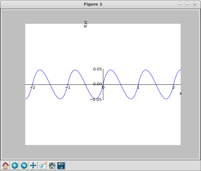
Fractional part

The fractional part of a non‐negative real number $x$ is the excess beyond that number’s integer part. If the latter is defined as the largest integer not greater than x, called floor of x or $\lfloor x\rfloor$ , its fractional part can be written as:

\operatorname {frac}(x)=x-\lfloor x\rfloor ,\;x>0

For a positive number written in a conventional positional numeral system (such as binary or decimal), its fractional part hence equals the digits appearing after the radix point.

For negative numbers

However, in case of negative numbers, there are various conflicting ways to extend the fractional part function to them: It is either defined in the same way as for positive numbers, i.e. by $\operatorname {frac}(x)=x-\lfloor x\rfloor$ (Graham, Knuth & Patashnik 1992),^[1] or as the part of the number to the right of the radix point, $\operatorname {frac}(x)=|x|-\lfloor |x|\rfloor$ (Daintith 2004),^[2] finally, by the odd function ^[3]

\operatorname {frac}(x)={\begin{cases}x-\lfloor x\rfloor &x\geq 0\\x-\lceil x\rceil &x<0\end{cases}}

with $\lceil x\rceil$ as the smallest integer not less than x, also called the ceiling of x. By consequence, we may get, for example, three different values for the fractional part of just one x: let it be −1.3, its fractional part will be 0.7 according to the first definition, 0.3 according to the second definition, and −0.3 according to the third definition, whose result can also be obtained in a straightforward way by

\operatorname {frac} (x)=x-\lfloor |x|\rfloor \cdot \operatorname {sgn}(x)

Unique decomposition into integer and fractional parts

Under the first definition all real numbers can be written in the form $n+r$ , where $n$ is the number to the left of the radix point, and the remaining fractional part $r$ is a nonnegative real number less than one. If $x$ is a positive rational number, then the fractional part of $x$ can be expressed in the form $p/q$ , where $p$ and $q$ are integers and $0\leq p<q$ . For example, if x = 1.05, then the fractional part of x is 0.05 and can be expressed as 5 / 100 = 1 / 20.

此處取捨之道無干『傳統』或『創新』，唯以容易畫圖︰

pi@raspberrypi:~ x - \lfloor x \rfloorfrac(x) = x - \lfloor x \rfloorB_1 (frac(x))B_2 (frac(x))B_3 (frac(x))$】

 
作者過去熟悉之符號選擇罷了。

FreeSandal

每月彙整: 2017 年 4 月

時間序列︰生成函數‧漸近展開︰當白努利遇上傅立葉《IV》

時間序列︰生成函數‧漸近展開︰當白努利遇上傅立葉《III》

費米悖論

悖論基礎

名字起源

Modal logic

勒貝格測度

問題起源

零測集

時間序列︰生成函數‧漸近展開︰當白努利遇上傅立葉《II》

Riemann zeta function

Definition

特殊函數

時間序列︰生成函數‧漸近展開︰當白努利遇上傅立葉《I》

傅立葉級數

歷史

定義

Integration by parts

Visualization

解析延拓

初步闡述

Fourier series

時間序列︰生成函數‧漸近展開︰當白努利遇上傅立葉《導言》

Periodic Bernoulli polynomials

Fractional part

For negative numbers

Unique decomposition into integer and fractional parts

輕。鬆。學。部落客

2017 年 4 月
日	一	二	三	四	五	六
« 3 月				5 月 »
						1
2	3	4	5	6	7	8
9	10	11	12	13	14	15
16	17	18	19	20	21	22
23	24	25	26	27	28	29
30