從牛頓力學來講,假使我們知道一個物體的『加速度』  ,而且如果『初始條件』︰該物位置在原點,速度為零。那麼任意時刻的『速度』是
  ,『位置』為
  。這麼簡易的算術有什麼重要嗎?若是我們可以『追跡物體 』,舉凡相機拍照的防震、手腳運動之練習、肢體平衡復健的監督﹐…… 實有著不勝枚舉之『用途』。然而『微機電』所作的『慣性感測器』 IMU ,一有免不了的『加速度』之『度量誤差』,此誤差在長『時間』的『積累』下將越來『錯誤』越大!再者那個『量測值』只能是『加速度』的『時間序列』
  ,因此
,因此  到
到  時刻間之事也就不得不有『假設』的了!!就像此處問答所說的一樣︰
Tracking 2D positioning with IMU Sensor
I am using a miniature car and I want to estimate the position. We can not use GPS modules and most of the tracking systems that I saw, are using IMU senson with the GPS module. In our car we are able to find our exact correct location with image processing but for some parts that dont have enough markings we can not do this. So we want to use the IMU as backup for our positioning. so as long as the positioning is close is good for us.
And we are only interested in our 2D position since the car is on a flat ground.
I am using a IMU 9DOF sensor and I want to calculate my movement. I have seen some amazing works with IMU for tracking body movements but no code or simple explanation is anywhere about it. So basically I have the reading from accelerometer, gyro and magnetometer. I also have orientation in quarternions. From the device I am getting also the linear acceleration but even when I am not moving it in any direction the values are not 0 which is really confusing.
Can you please help me how to approach this?
Thanks in advance
Update :
So right now we are getting the perfect heading from the quaternion values. We also have the delta_time between each heading. So what I believe we need right now is the velocity. either as a vector or as a total value.
───
Non-zero rates are normal for MEMS accelerometers and gyros. This is persistent error. It is eliminated by somehow making sure that the device is stationary for a couple of seconds (so the output can stabilize), then getting a reading. Henceforth, subtracting this steady-state error from all future measurements. Look up the datasheet of your sensor – there will be maximum values for this and other types of measurement tolerances.
Now, the much more complex subject of fusing the accelerometer, gyro and compass data. This can get hugely complicated, using Kalman filter, like Apolo once did. It can, however, be quite simple as well.
The general idea is that the magnetic sensor has slow response, low accuracy, but the error does not increase. On the other hand, a gyro’s output is velocity, which is integrated to get angular position. The error grows very fast – generally you can’t do dead reckoning for more than a minute with only a giro. The accelerometer is worse – it outputs acceleration, which gets integrated twice!
So, a simple fusing filter would be some linear combination of the readings of the accelerometer and compass, with the coefficient in front of the gyro descreasing over tyme.
Here is a discussion by much more knowledgeable people than me on the topic.
Note: What you are trying to do is called dead reckoning.
───
於是為了能夠更好的『應用』 IMU ,終將走入『數據處理』之路。『卡爾曼濾波』 Kalman filter
Kalman filtering, also known as linear quadratic estimation (LQE), is an algorithm that uses a series of measurements observed over time, containing statistical noise and other inaccuracies, and produces estimates of unknown variables that tend to be more precise than those based on a single measurement alone. The filter is named after Rudolf E. Kálmán, one of the primary developers of its theory.
The Kalman filter has numerous applications in technology. A common application is for guidance, navigation and control of vehicles, particularly aircraft and spacecraft. Furthermore, the Kalman filter is a widely applied concept in time series analysis used in fields such as signal processing and econometrics. Kalman filters also are one of the main topics in the field of robotic motion planning and control, and they are sometimes included in trajectory optimization. The multi-fractional order estimator is a simple and practical alternative to the Kalman filter for tracking targets.
The algorithm works in a two-step process. In the prediction step, the Kalman filter produces estimates of the current state variables, along with their uncertainties. Once the outcome of the next measurement (necessarily corrupted with some amount of error, including random noise) is observed, these estimates are updated using a weighted average, with more weight being given to estimates with higher certainty. The algorithm is recursive. It can run in real time, using only the present input measurements and the previously calculated state and its uncertainty matrix; no additional past information is required.
The Kalman filter does not require any assumption that the errors are Gaussian.[1] However, the filter yields the exact conditional probability estimate in the special case that all errors are Gaussian-distributed.
Extensions and generalizations to the method have also been developed, such as the extended Kalman filter and the unscented Kalman filter which work on nonlinear systems. The underlying model is a Bayesian model similar to a hidden Markov model but where the state space of the latent variables is continuous and where all latent and observed variables have Gaussian distributions.
……
就是早年發展重要的一種『數據處理』方法。也許下面一篇論文的『摘要』
Abstract
This paper investigates two methods of displacement estimation using sampled acceleration and orientation data from a 6 degrees of freedom (DOF) Inertial Measurement Unit (IMU), with the application to sporting training and rehabilitation. Currently, the use of low cost IMUs for this particular application is very impractical due to the accumulation of errors from various sources. Previous studies and projects that have applied IMUs to similar applications have used a lower number of DOF, or have used higher accuracy navigational grade IMUs. Solutions to the acceleration noise accumulation and gyroscope angle error problem are proposed in this paper. A zero velocity update algorithm (ZUPT) is also developed to improve the accuracy of displacement estimation with a low grade IMU. The experimental results from this study demonstrate the feasibility of using an IMU with loose tolerances to determine the displacement. Peak distances of a range of exercises are shown to be measured with accuracies within 5% for the numerical integration methods.
Keywords
estimation, profile, displacement, sporting, applications, sensors, motion, inertial, exercises, cost, rehabilitation, low
Disciplines
Engineering | Science and Technology Studies
Publication Details
J. Coyte, D. A. Stirling, M. Ros, H. Du & A. Gray, “Displacement profile estimation using low cost inertial motion sensors with applications to sporting and rehabilitation exercises,” in 2013 IEEE/ASME International Conference on Advanced Intelligent Mechatronics (AIM), 2013, pp. 1290-1295.
───
將引領我們走得更遠乎??終究莫忘那『微分』與『差分』方程式可以很不相同的耶!!


相圖

定點‧震盪‧混沌
一八三八年,比利時數學家 Pierre François Verhulst 發表了一個『人口成長』方程式,

,此處  是某時的人口數,
 是自然成長率,
  是環境承載力。求解後得到

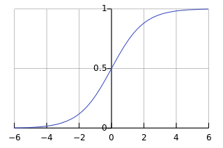
,此處  是初始條件。 Verhulst 將這個函數稱作『logistic function』,於是那個微分方程式也就叫做『 logistic equation』。假使用
  改寫成
改寫成  ,將它『標準化』,取
  與
與  ,從左圖的解答來看,
  ,也就是講人口數成長不可能超過環境承載力的啊!
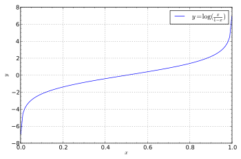
如果求  的反函數,得到
  ,這個反函數被稱之為『Logit』函數,定義為

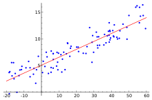
,一般常用於『二元選擇』,比方說『To Be or Not To Be』的『機率分佈』,也用於『迴歸分析』 Regression Analysis 來看看兩個『變量』在統計上是『相干』還是『無干』的ㄡ!假使試著用『無窮小』 數來看  和
和  ,或許更能體會『兩極性』的吧!!
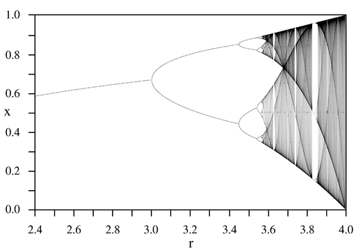
一九七六年,澳洲科學家 Robert McCredie May 發表了一篇《Simple mathematical models with very complicated dynamics》文章,提出了一個『單峰映象』 logistic map 遞迴關係式  。這個遞迴關係式很像是『差分版』的『 logistic equation』,竟然是產生『混沌現象』的經典範例。假使說一個『遞迴關係式』有『極限值』
 的話,此時
的話,此時  ,可以得到
,可以得到  ,於是
,於是  或者
或者  。在
。在  之時,『單峰映象』或快或慢的收斂到『零』; 當
  之時,它很快的逼近
  ;於
;於  之時,線性的上下震盪趨近 ;雖然
  也收斂到 ,然而已經是很緩慢而且不是線性的了;當
  時,對幾乎各個『初始條件』而言,系統開始發生兩值『震盪現象』,而後變成四值、八值、十六值…等等的『持續震盪』;最終於大約
  時,這個震盪現象消失了,系統就步入了所謂的『混沌狀態』的了!!
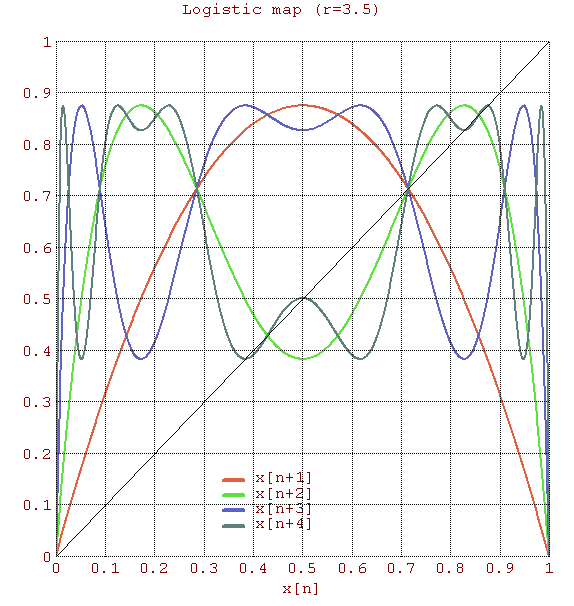
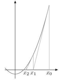
『連續的』微分方程式沒有『混沌性』,『離散的』差分方程式反倒發生了『混沌現象』,那麼這個『量子』的『宇宙』到底是不是『混沌』的呢??回想之前『λ 運算』裡的『遞迴函式』,與數學中的『定點』定義,『單峰映象』可以看成函數  的『迭代求值』︰
 。當
。當  ,這個
,這個  就是『定點』,左圖中顯示出不同的 值的求解現象,從有『定點』向『震盪』到『混沌』。如果我們將『 logistic equation』 改寫成
 ![\Delta P(t) = P(t + \Delta t) - P(t) = \left( r P(t) \left[ 1 - P(t) \right] \right) \cdot \Delta t](http://www.freesandal.org/wp-content/ql-cache/quicklatex.com-f862e9b7a6f8941170eb4a06470c1d45_l3.png "Rendered by QuickLaTeX.com") ,假使取
,假使取  ,可以得到
,可以得到 ![P(n + 1) - P(n) = r P(n) \left[ 1 - P(n) \right]](http://www.freesandal.org/wp-content/ql-cache/quicklatex.com-a2bcd9e1f12ec10b81e56b84b4810ef4_l3.png "Rendered by QuickLaTeX.com") ,它的『極限值』
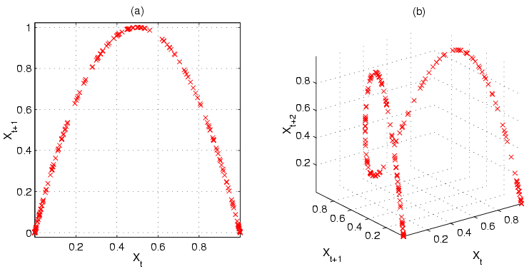
,它的『極限值』  ,根本與 沒有關係,這也就說明了兩者的『根源』是不同的啊!然而這卻建議著一種『時間序列』的觀點,如將
  看成
看成  ,這樣
,這樣 ![\frac{x[(n+1) \Delta t] - x[n \Delta t]}{\Delta t} = x_{n+1} - x_n](http://www.freesandal.org/wp-content/ql-cache/quicklatex.com-099817979576eb719a1d1161a407d71d_l3.png "Rendered by QuickLaTeX.com") 就說是『速度』的了,於是
就說是『速度』的了,於是  便構成了假想的『相空間』,這可就把一個『遞迴關係式』轉譯成了一種『符號動力學』的了!!
在某些特定的 值,這個『遞迴關係式』有『正確解』 exact solution,比方說  時,
時, ,因為
,因為  ,所以
,所以  ,於是
,於是  ,因此
,因此  。再者由於『指數項』
  是『偶數』,所以此『符號動力系統』不等速 ── 非線性 ── 而且不震盪的逼近『極限值』的啊。
對於  來講,它的解是

,此處  是『初始條件』參數,可由
  來決定。假使 是『有理數』,那麼
  這個『周期函數』,多次『迭代』後就可能產生『極限循環』;要是 是『無理數』,它有一個『不循環』的無窮小數成份,這個『符號動力系統』就彷彿是『隨機亂動』一般,因此才說它是『混沌』的啊!假使思考 是一個『有理數』的機會,怕是很渺茫的吧!!
── 引自《【Sonic π】電路學之補充《四》無窮小算術‧中下上》