時間序列︰生成函數‧漸近展開︰白努利 □○《六》

2017-03-26 懸鉤子

水滸傳　　元(明) ‧ 施耐庵輯

第十六回　楊志押送金銀擔　吳用智取生辰綱

話說當時公孫勝正在閣兒裏對晁蓋說這北京「生辰綱」是不義之財，取之何礙。只見一個人從外面搶將入來，揪住公孫勝道：「你好大膽！卻才商議的事，我都知了也。」那人卻是「智多星」吳學究。晁蓋笑道：「教授休慌，且請相見。」兩個敘禮罷。吳用道：「江湖上久聞人說『入雲龍』公孫勝一清大名，不期今日此處得會！」晁蓋道：「這位秀才先生，便是『智多星』吳學究。」公孫勝道：「吾聞江湖上多人曾說加亮先生大名，豈知緣法卻在保正莊上得會。只是保正疏財仗義，以此天下豪傑，都投門下。」晁蓋道：「再有幾個相識在裏面，一發請進後堂深處相見。」三個人入到裏面，就與劉唐、三阮都相見了。正是：

金帛多藏禍有基，英雄聚會本無期。一時豪俠欺黃屋，七宿光芒動紫薇。

………

生成函數有何『用』？無『用』處『用』是『大用』？？『用大』之道可尋味！

老子第四十二章中講︰道生一，一生二，二生三，三生萬物。是說天地生萬物就像四季循環的自然而然，如果『人』或將成為『亦大』，就得知道大自然『益』生之道，能循本溯源貴能『得一』。他固善於『觀水』，盛讚『上善若水』，卻也深知水為山堵之『蹇』、人為慾阻之『蒙』難，故於第三十九章中又講︰

昔之得一者，天得一以清，地得一以寧，神得一以靈，谷得一以盈，萬物得一以生，侯王得一以為天下貞。其致之。天無以清則恐裂，地無以寧則恐發，神無以靈則恐歇，谷無以盈則恐竭，萬物無以生則恐滅，侯王無以貞高則恐蹶。故貴以賤為本，高以下為基。是以侯王自謂孤寡不穀，此非以賤為本耶？非乎？人之所惡 ，唯孤寡不穀，而侯王以為稱。故致譽無譽。不欲琭琭如玉，珞珞如石。

，希望人們知道所謂『道德』之名，實在說的是『得到』── 得道── 的啊！！如果乾坤都『沒路』可走，人又該往向『何方』？？

昔時吳越之爭，越王勾踐『臥薪嘗膽』逐夢復國，此事紀載於《史記‧越王勾踐世家》，在此我們將談及一人亦載之於史記︰

范蠡‧史記‧貨殖列傳

昔者越王句踐困於會稽之上，乃用范蠡、計然。計然曰：『知斗則修備，時用則知物，二者形則萬貨之情可得而觀已。故歲在金，穰；水，毀；木，饑；火，旱。旱則資舟，水則資車，物之理也 。六歲穰，六歲旱，十二歲一大饑。夫糶，二十病農，九十病末。末病則財不出，農病則草不辟矣。上不過八十，下不減三十，則農末俱利，平糶齊物，關市不乏，治國之道也。積著之理，務完物，無息幣。以物相貿易，腐敗而食之貨勿留，無敢居貴。 論其有餘不足，則知貴賤。貴上極則反賤，賤下極則反貴。貴出如糞土，賤取如珠玉。財幣欲其行如流水。』修之十年，國富，厚賂戰士，士赴矢石，如渴得飲，遂報彊吳，觀兵中國，稱號『五霸』。

范蠡既雪會稽之恥，乃喟然而嘆曰：「計然之策七，越用其五而得意。既已施於國，吾欲用之家。」乃乘扁舟浮於江湖，變名易姓 ，適齊為鴟夷子皮，之陶為朱公。 朱公以為陶天下之中，諸侯四通，貨物所交易也。乃治產積居。與時逐而不責於人。故善治生者，能擇人而任時。十九年之中三致千金，再分散與貧交疏昆弟。此所謂富好行其德者也。後年衰老而聽子孫，子孫修業而息之，遂至巨萬。故言富者皆稱陶朱公。

文子治國富民之策有七，越王只用其五就洋洋得意。范蠡細省已用『天時』、『地利』二者，所餘不用，不就是『人和』不用了嗎？勾踐得國後必將失人，此時不乘扁舟浮於江湖，怕我連命都不保了。陶朱公之為後世所稱的『財神』，不因他能得之於天下成大富巨萬，而因他能『三聚三散』用之於天下。此時如果再讀讀莊子的二則寓言︰

莊子‧胠篋之竊鉤者誅，竊國者為諸侯；

聖人不死，大盜不止。雖重聖人而治天下，則是重利盜跖也。為之斗斛以量之，則並與斗斛而竊之；為之權衡以稱之，則並與權衡而竊之；為之符璽以信之，則並與符璽而竊之；為之仁義以矯之，則並與仁義而竊之。何以知其然邪？彼竊鉤者誅，竊國者為諸侯，諸侯之門而仁義存焉，則是非竊仁義聖知邪？故逐於大盜，揭諸侯，竊仁義並斗斛權衡符璽之利者，雖有軒冕之賞弗能勸，斧鉞之威弗能禁。此重利盜跖而使不禁者，是乃聖人之過也。

莊子‧秋水之無用用大；

惠子謂莊子曰：魏王貽我大瓠之種，我樹之成而實五石。以盛水漿，其堅不能自舉也；剖之以為瓢，則瓠落無所容。非不呺然大也，吾為其無用而掊之。

莊子曰：夫子固拙于用大矣！宋人有善為不龜手之藥者，世世以洴澼絖為事。客聞之，請買其方百金。聚族而謀曰：『我世世為洴澼絖，不過數金，今一朝而鬻技百金，請與之。』客得之，以說吳王。越有難，吳王使之將。冬，與越人水戰，大敗越人，裂地而封之。能不龜手一也；或以封，或不免於洴澼絖，則所用之異也。今子有五石之瓠，何不慮以為大樽，而浮於江湖，而憂其瓠落無所容？則夫子猶有蓬之心也夫！

─── 摘自《跟隨□？築夢！！》

氣味相投可『言小』！！『用小』之術胡可說？氣息就在呼吸間，履霜堅冰循自然，水滴石穿豈無期！！好高騖遠乏基石，怎得花開月圓時？？大小內外皆天地☆

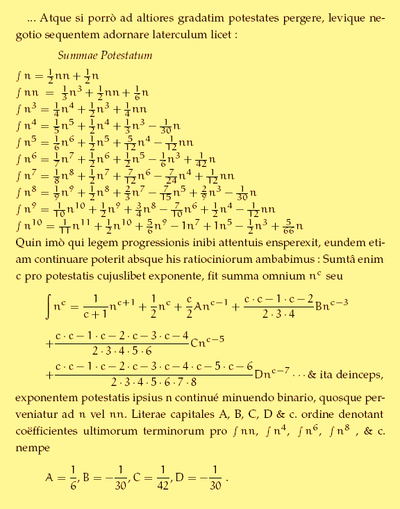
既得白努利數之生成函數 $G(t) = \frac{t}{e^t -1}$ 且先探其奇偶性乎？

Even and odd functions

In mathematics, even functions and odd functions are functions which satisfy particular symmetry relations, with respect to taking additive inverses. They are important in many areas of mathematical analysis, especially the theory of power series and Fourier series. They are named for the parity of the powers of the power functions which satisfy each condition: the function f(x) = xⁿ is an even function if n is an even integer, and it is an odd function if n is an odd integer.

Definition and examples

The concept of evenness or oddness is defined for functions whose domain and image both have an additive inverse. This includes additive groups, all rings, all fields, and all vector spaces. Thus, for example, a real-valued function of a real variable could be even or odd, as could a complex-valued function of a vector variable, and so on.

The examples are real-valued functions of a real variable, to illustrate the symmetry of their graphs.

Even functions

ƒ(x) = x² is an example of an even function.

Let f(x) be a real-valued function of a real variable. Then f is even if the following equation holds for all x and -x in the domain of f:^[1]

f(x) = f(-x), \,

f(x) - f(-x) = 0. \,

Geometrically speaking, the graph face of an even function is symmetric with respect to the y-axis, meaning that its graph remains unchanged after reflection about the y-axis.

Examples of even functions are |x|, x², x⁴, cos(x), cosh(x), or any linear combination of these.

Odd functions

ƒ(x) = x³ is an example of an odd function.

Again, let f(x) be a real-valued function of a real variable. Then f is odd if the following equation holds for all x and -x in the domain of f:^[2]

-f(x) = f(-x), \,

f(x) + f(-x) = 0. \,

Geometrically, the graph of an odd function has rotational symmetry with respect to the origin, meaning that its graph remains unchanged after rotation of 180 degrees about the origin.

Examples of odd functions are x, x³, sin(x), sinh(x), erf(x), or any linear combination of these.

$G(-t) = \frac{-t}{e^{-t} - 1} = \frac{t}{1 -e^{-t}} = e^t G(t)$ 雖然非奇非偶，此形式 $\frac{1}{1 - e^{-t}}$ 數理直通光明道︰

Bose–Einstein statistics

In quantum statistics, Bose–Einstein statistics (or more colloquially B–E statistics) is one of two possible ways in which a collection of non-interacting indistinguishable particles may occupy a set of available discrete energy states, at thermodynamic equilibrium. The aggregation of particles in the same state, which is a characteristic of particles obeying Bose–Einstein statistics, accounts for the cohesive streaming of laser light and the frictionless creeping of superfluid helium. The theory of this behaviour was developed (1924–25) by Satyendra Nath Bose, who recognized that a collection of identical and indistinguishable particles can be distributed in this way. The idea was later adopted and extended by Albert Einstein in collaboration with Bose.

The Bose–Einstein statistics apply only to those particles not limited to single occupancy of the same state—that is, particles that do not obey the Pauli exclusion principle restrictions. Such particles have integer values of spin and are named bosons, after the statistics that correctly describe their behaviour. There must also be no significant interaction between the particles.

Derivation from the grand canonical ensemble

The Bose–Einstein distribution, which applies only to a quantum system of non-interacting bosons, is easily derived from the grand canonical ensemble.^[3] In this ensemble, the system is able to exchange energy and exchange particles with a reservoir (temperature T and chemical potential µ fixed by the reservoir).

Due to the non-interacting quality, each available single-particle level (with energy level ϵ) forms a separate thermodynamic system in contact with the reservoir. In other words, each single-particle level is a separate, tiny grand canonical ensemble. With bosons there is no limit on the number of particles N in the level, but due to indistinguishability each possible N corresponds to only one microstate (with energy Nϵ). The resulting partition function for that single-particle level therefore forms a geometric series:

{\begin{aligned}{\mathcal {Z}}&=\sum _{N=0}^{\infty }\exp(N(\mu -\epsilon )/k_{B}T)=\sum _{N=0}^{\infty }[\exp((\mu -\epsilon )/k_{B}T)]^{N}\\&={\frac {1}{1-\exp((\mu -\epsilon )/k_{B}T)}}\end{aligned}}

and the average particle number for that single-particle substate is given by

\langle N\rangle =k_{B}T{\frac {1}{\mathcal {Z}}}\left({\frac {\partial {\mathcal {Z}}}{\partial \mu }}\right)_{V,T}={\frac {1}{\exp((\epsilon -\mu )/k_{B}T)-1}}

This result applies for each single-particle level and thus forms the Bose–Einstein distribution for the entire state of the system.^[4]^[5]

The variance in particle number (due to thermal fluctuations) may also be derived:

\langle (\Delta N)^{2}\rangle =k_{B}T\left({\frac {d\langle N\rangle }{d\mu }}\right)_{V,T}=\langle N^{2}\rangle -\langle N\rangle ^{2}

This level of fluctuation is much larger than for distinguishable particles, which would instead show Poisson statistics $\langle (\Delta N)^{2}\rangle =\langle N\rangle ^{2}$ ). This is because the probability distribution for the number of bosons in a given energy level is a geometric distribution, not a Poisson distribution.

發現過程原錯誤，

History

While presenting a lecture at the University of Dhaka on the theory of radiation and the ultraviolet catastrophe, Satyendra Nath Bose intended to show his students that the contemporary theory was inadequate, because it predicted results not in accordance with experimental results. During this lecture, Bose committed an error in applying the theory, which unexpectedly gave a prediction that agreed with the experiment. The error was a simple mistake—similar to arguing that flipping two fair coins will produce two heads one-third of the time—that would appear obviously wrong to anyone with a basic understanding of statistics (remarkably, this error resembled the famous blunder by d’Alembert known from his “Croix ou Pile” Article). However, the results it predicted agreed with experiment, and Bose realized it might not be a mistake after all. For the first time, he took the position that the Maxwell–Boltzmann distribution would not be true for all microscopic particles at all scales. Thus, he studied the probability of finding particles in various states in phase space, where each state is a little patch having volume h³, and the position and momentum of the particles are not kept particularly separate but are considered as one variable.

Bose adapted this lecture into a short article called “Planck’s Law and the Hypothesis of Light Quanta”^[1]^[2] and submitted it to the Philosophical Magazine. However, the referee’s report was negative, and the paper was rejected. Undaunted, he sent the manuscript to Albert Einstein requesting publication in the Zeitschrift für Physik. Einstein immediately agreed, personally translated the article from English into German (Bose had earlier translated Einstein’s article on the theory of General Relativity from German to English), and saw to it that it was published. Bose’s theory achieved respect when Einstein sent his own paper in support of Bose’s to Zeitschrift für Physik, asking that they be published together. This was done in 1924.

The reason Bose produced accurate results was that since photons are indistinguishable from each other, one cannot treat any two photons having equal energy as being two distinct identifiable photons. By analogy, if in an alternate universe coins were to behave like photons and other bosons, the probability of producing two heads would indeed be one-third, and so is the probability of getting a head and a tail which equals one-half for the conventional (classical, distinguishable) coins. Bose’s “error” leads to what is now called Bose–Einstein statistics.

Bose and Einstein extended the idea to atoms and this led to the prediction of the existence of phenomena which became known as Bose–Einstein condensate, a dense collection of bosons (which are particles with integer spin, named after Bose), which was demonstrated to exist by experiment in 1995.

莫非天使遣之說？？！！光子處處無不在，白努利數時時現身來！！？？皆住空無妙有宅☆

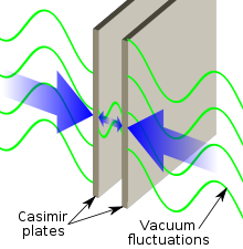
一九四八年時，荷蘭物理學家『亨德里克‧卡西米爾』 Hendrik Casimir 提出了『真空不空』的『議論』。因為依據『量子場論』，『真空』也得有『最低能階』，因此『真空能量』不論因不因其『實虛』粒子之『生滅』，總得有一個『量子態』。由於已知『原子』與『分子』的『主要結合力』是『電磁力』，那麼該『如何』說『真空』之『量化』與『物質』的『實際』是怎麽來『配合』的呢？因此他『計算』了這個『可能效應』之『大小』，然而無論是哪種『震盪』所引起的，他總是得要面臨『無窮共振態』 $\langle E \rangle = \frac{1}{2} \sum \limits_{n}^{\infty} E_n$ 的『問題』，這也就是說『平均』有『多少』各種能量的『光子？』所參與 $h\nu + 2h\nu + 3h\nu + \cdots$ 的『問題』？據知『卡西米爾』用『歐拉』等之『可加法』，得到了 ${F_c \over A} = -\frac {\hbar c \pi^2} {240 a^4}$ 。

此處之『負』 $-$ 代表『吸引力』，而今早也已經『證實』的了，真不知『宇宙』是果真先就有『計畫』的嗎？還是說『人們』自己還在『幻想』的呢？？

─── 摘自《【Sonic π】電聲學之電路學《四》之《 V!》‧下》

關係一現機鋒出 $G(-t) - G(t) = e^t G(t) - G(t) = t$ 。原來這個白努利數唯一奇 $B_1$ ， $- B_1 - B_1 = 1$ ，不假它求數自知 $B_1 = -\frac{1}{2}$ 。遞迴關係無覓處

$(m+1) B_m = - \sum \limits_{k=0}^{m-1} \left( \begin{array}{ccc} m+1 \\ k \end{array} \right) B_k$

。恰恰此中得

$t = \sum \limits_{m=0}^{\infty} B_m \frac{t^m}{m !} \cdot (e^t -1)$

☆

樹莓派、樹莓派之學習、樹莓派之教育

時間序列︰生成函數‧漸近展開︰白努利 □○《五》

2017-03-25 懸鉤子

數理論述若是簡單易明恐有掛一漏萬之失，複雜難解常生白馬非馬之病。蓋因為概念間單行、雙向蘊涵之邏輯網，前前後後密密麻麻，上上下下難知何為本何為末！！圜圜回回怎曉哪是頭哪是尾？？此所以數學之惱人也。然而本末頭尾全是練習而來，書籍文章不過編織材料，自造學問之網自得之乎？倘有病失不在知識之過耶！

且讓我們借著等冪求和生成函數

$\sum \limits_{p=0}^{\infty} S_p(n-1) \frac{x^p}{p !} = \sum \limits_{p = 0}^\infty \left({\sum \limits_{k = 0}^{n - 1} k^p}\right) \frac {x^p} {p!} = \sum \limits_{k = 0}^{n - 1} e^{k x} = \frac {e^{n x} - 1} {e^x - 1} = G(x)$

起頭，談談操作自修吧！

首先

$S_0(n-1) = 0^0 + 1^0 + \cdots + {(n-1)}^0 = n$ ，但

$G(0) = \frac {e^{n \cdot 0} - 1 } {e^0 - 1} = \frac{0}{0}$ ，所以得用 L’Hôpital’s rule

$G(0) = \lim \limits_{x \to 0} \frac {e^{n x} - 1} {e^x - 1} = \lim \limits_{x \to 0} \frac{n e^{n x}}{e^x} = n$ 。

那麼 $S_1(n-1) = 0^1 + 1^1 + \cdots + {(n-1)}^1 = \frac{n (n-1)}{2}$ 是否等於 $\lim \limits_{x \to 0} \frac{dG(x)}{d x} = \lim \limits_{x \to 0} G^{'} (x)$ 呢？

$G^{'} (x) = {\left( \frac{e^{n x} - 1}{e^x - 1} \right)}^{'} = \frac{n e^{n x}}{e^x -1} - \frac{e^x (e^{n x} -1)}{{(e^x - 1)}^2}$

$= \frac{(n-1) e^x e^{nx} - n e^{nx} + e^x} {{(e^x - 1)}^2}, \ \to \frac{(n-1) - n +1}{0} = \frac{0}{0}$ 。由於

${\left( (n-1) e^x e^{nx} - n e^{nx} + e^x \right)}{'} = (n-1)(e^x e^{nx} + n e^x e^{nx}) - n^2 e^{nx} + e^x ,$

$\to (n-1) + n(n-1) - n^2 + 1 = 0$

${\left( {(e^x - 1)}^2 \right)}^{'} = 2 (e^x - 1) e^x, \ \to 0$

${\left( (n-1) e^x e^{nx} - n e^{nx} + e^x \right)}{''}$

$= (n-1) e^x e^{nx} + 2 n (n-1) e^x e^{nx} + n^2 (n-1) e^x e^{nx} - n^3 e^{nx} + e^x,$

$\to (n-1) + 2 n (n-1) + n^2 (n-1) - n^3 + 1 = n^2 - n$

${\left( {(e^x - 1)}^2 \right)}^{''} = 2 e^x (2 e^x - 1), \to 2$

$\therefore \lim \limits_{x \to 0} G^{'} (x) = \frac{n^2 - n}{2} = S_1(n-1)$ 。

莫笑作者癡，分明已有好工具︰

pi@raspberrypi:~ \frac{0}{0}x = 0e^{nx} - 1 = \sum \limits_{k=1}^{\infty} \frac{{(nx)}^k}{k !}e^{x} - 1 = \sum \limits_{k=1}^{\infty} \frac{x^k}{k !}\frac{1}{e^{x} - 1}B_0 = 1B_0\lim \limits_{x \to 0} G_B(x) = 1\frac{\alpha \cdot x}{e ^x -1}\lim \limits_{x \to 0} \frac{\alpha \cdot x}{e ^x -1} = \lim \limits_{x \to 0} \frac{\alpha}{e^x}  = \alpha = 1 $ 了☆

樹莓派、樹莓派之學習、樹莓派之教育

時間序列︰生成函數‧漸近展開︰白努利 □○《四》

2017-03-24 懸鉤子

白努利數起源於等冪求和公式

Faulhaber’s formula

Theorem

Let n and p be positive integers.

Then:

$\sum \limits_{k = 1}^n k^p = \frac 1 {p + 1} \sum \limits_{i = 0}^p \left({-1}\right)^i \binom {p + 1} i B_i n^{p + 1 - i}$

where Bn denotes the nth Bernoulli number.

之符號通解的追求應無疑議。

從白努利《Ars Conjectandi》書中的形式表述看來

Reconstruction of “Summae Potestatum“

Jakob Bernoulli’s Summae Potestatum, 1713

The Bernoulli numbers were introduced by Jakob Bernoulli in the book Ars Conjectandi published posthumously in 1713 page 97. The main formula can be seen in the second half of the corresponding facsimile. The constant coefficients denoted $A$ , $B$ , $C$ and $D$ by Bernoulli are mapped to the notation which is now prevalent as $A = B 2$ , $B = B 4$ , $C = B 6$ , $D = B 8$ . The expression $c \cdot c -1\cdot c -2\cdot c -3$ means $c \cdot(c -1)\cdot(c -2)\cdot(c -3)$ – the small dots are used as grouping symbols. Using today’s terminology these expressions are falling factorial powers $c k$ . The factorial notation $k!$ as a shortcut for $1 \times 2 \times \dots \times k$ was not introduced until 100 years later. The integral symbol on the left hand side goes back to Gottfried Wilhelm Leibniz in 1675 who used it as a long letter $S$ for “summa” (sum). (The Mathematics Genealogy Project^[14] shows Leibniz as the doctoral adviser of Jakob Bernoulli. See also the Earliest Uses of Symbols of Calculus.^[15]) The letter $n$ on the left hand side is not an index of summation but gives the upper limit of the range of summation which is to be understood as $1, 2, \dots, n$ . Putting things together, for positive $c$ , today a mathematician is likely to write Bernoulli’s formula as:

\sum _{k=1}^{n}k^{c}={\frac {n^{c+1}}{c+1}}+{\frac {1}{2}}n^{c}+\sum _{k=2}^{\infty }{\frac {B_{k}}{k!}}c^{\underline {k-1}}n^{c-k+1}.

In fact this formula imperatively suggests to set $B 1 = 1 / 2$ when switching from the so-called ‘archaic’ enumeration which uses only the even indices 2, 4, 6… to the modern form (more on different conventions in the next paragraph). Most striking in this context is the fact that the falling factorial $c k -1$ has for $k = 0$ the value $\frac{1}{c+1}$ .^[16] Thus Bernoulli’s formula can and has to be written

\sum _{k=1}^{n}k^{c}=\sum _{k=0}^{\infty }{\frac {B_{k}}{k!}}c^{\underline {k-1}}n^{c-k+1}

if $B 1$ stands for the value Bernoulli himself has given to the coefficient at that position.

恐尚未能將白努利數看成數列吧！何況泰勒級數

Taylor series

History

The Greek philosopher Zeno considered the problem of summing an infinite series to achieve a finite result, but rejected it as an impossibility: the result was Zeno’s paradox. Later, Aristotle proposed a philosophical resolution of the paradox, but the mathematical content was apparently unresolved until taken up by Archimedes, as it had been prior to Aristotle by the Presocratic Atomist Democritus. It was through Archimedes’s method of exhaustion that an infinite number of progressive subdivisions could be performed to achieve a finite result.^[1] Liu Hui independently employed a similar method a few centuries later.^[2]

In the 14th century, the earliest examples of the use of Taylor series and closely related methods were given by Madhava of Sangamagrama.^[3]^[4] Though no record of his work survives, writings of later Indian mathematicians suggest that he found a number of special cases of the Taylor series, including those for the trigonometric functions of sine, cosine, tangent, and arctangent. The Kerala school of astronomy and mathematics further expanded his works with various series expansions and rational approximations until the 16th century.

In the 17th century, James Gregory also worked in this area and published several Maclaurin series. It was not until 1715 however that a general method for constructing these series for all functions for which they exist was finally provided by Brook Taylor,^[5] after whom the series are now named.

The Maclaurin series was named after Colin Maclaurin, a professor in Edinburgh, who published the special case of the Taylor result in the 18th century.

之發展，直到一七一五年方可稱完整。再從歐拉

Leonhard Euler

對數學分析的貢獻，及與白努利家族之情誼講起︰

Analysis

The development of infinitesimal calculus was at the forefront of 18th century mathematical research, and the Bernoullis—family friends of Euler—were responsible for much of the early progress in the field. Thanks to their influence, studying calculus became the major focus of Euler’s work. While some of Euler’s proofs are not acceptable by modern standards of mathematical rigour^[34] (in particular his reliance on the principle of the generality of algebra), his ideas led to many great advances. Euler is well known in analysis for his frequent use and development of power series, the expression of functions as sums of infinitely many terms, such as

e^{x}=\sum _{n=0}^{\infty }{x^{n} \over n!}=\lim _{n\to \infty }\left({\frac {1}{0!}}+{\frac {x}{1!}}+{\frac {x^{2}}{2!}}+\cdots +{\frac {x^{n}}{n!}}\right).

Notably, Euler directly proved the power series expansions for $e$ and the inverse tangent function. (Indirect proof via the inverse power series technique was given by Newton and Leibniz between 1670 and 1680.) His daring use of power series enabled him to solve the famous Basel problem in 1735 (he provided a more elaborate argument in 1741):^[34]

\sum _{n=1}^{\infty }{1 \over n^{2}}=\lim _{n\to \infty }\left({\frac {1}{1^{2}}}+{\frac {1}{2^{2}}}+{\frac {1}{3^{2}}}+\cdots +{\frac {1}{n^{2}}}\right)={\frac {\pi ^{2}}{6}}.

A geometric interpretation of Euler’s formula

Euler introduced the use of the exponential function and logarithms in analytic proofs. He discovered ways to express various logarithmic functions using power series, and he successfully defined logarithms for negative and complex numbers, thus greatly expanding the scope of mathematical applications of logarithms.^[32] He also defined the exponential function for complex numbers, and discovered its relation to the trigonometric functions. For any real number $φ$ (taken to be radians), Euler’s formula states that the complex exponential function satisfies

e^{i\varphi }=\cos \varphi +i\sin \varphi .\,

A special case of the above formula is known as Euler’s identity,

e^{i\pi }+1=0\,

called “the most remarkable formula in mathematics” by Richard P. Feynman, for its single uses of the notions of addition, multiplication, exponentiation, and equality, and the single uses of the important constants 0, 1, $e$ , $i$ and $π$ .^[35] In 1988, readers of the Mathematical Intelligencer voted it “the Most Beautiful Mathematical Formula Ever”.^[36] In total, Euler was responsible for three of the top five formulae in that poll.^[36]

De Moivre’s formula is a direct consequence of Euler’s formula.

In addition, Euler elaborated the theory of higher transcendental functions by introducing the gamma function and introduced a new method for solving quartic equations. He also found a way to calculate integrals with complex limits, foreshadowing the development of modern complex analysis. He also invented the calculus of variations including its best-known result, the Euler–Lagrange equation.

Euler also pioneered the use of analytic methods to solve number theory problems. In doing so, he united two disparate branches of mathematics and introduced a new field of study, analytic number theory. In breaking ground for this new field, Euler created the theory of hypergeometric series, q-series, hyperbolic trigonometric functions and the analytic theory of continued fractions. For example, he proved the infinitude of primes using the divergence of the harmonic series, and he used analytic methods to gain some understanding of the way prime numbers are distributed. Euler’s work in this area led to the development of the prime number theorem.^[37]

白努利數之生成函數 $\frac{x}{e^x -1} = \sum \limits_{k=0}^{\infty} B_k \frac{x^k}{k !}$ 或出自歐拉之手乎？否則哪來的一七三五年之歐拉-麥克勞林求和公式耶！！？？

Euler–Maclaurin formula

In mathematics, the Euler–Maclaurin formula provides a powerful connection between integrals (see calculus) and sums. It can be used to approximate integrals by finite sums, or conversely to evaluate finite sums and infinite series using integrals and the machinery of calculus. For example, many asymptotic expansions are derived from the formula, and Faulhaber’s formula for the sum of powers is an immediate consequence.

The formula was discovered independently by Leonhard Euler and Colin Maclaurin around 1735 (and later generalized as Darboux’s formula). Euler needed it to compute slowly converging infinite series while Maclaurin used it to calculate integrals.

……

The formula is often written with the subscript taking only even values, since the odd Bernoulli numbers are zero except for $B_{1},$ in which case we have ^[1]^[2]

\sum _{i=m+1}^{n}f(i)=\int _{m}^{n}f(x)\,dx+{\frac {f(n)-f(m)}{2}}+\sum _{k=1}^{\lfloor p/2\rfloor }{\frac {B_{2k}}{(2k)!}}(f^{(2k-1)}(n)-f^{(2k-1)}(m))+R.

───

誠如柯西之所言，『代數的普適性』

Generality of algebra

In the history of mathematics, the generality of algebra was a phrase used by Augustin-Louis Cauchy to describe a method of argument that was used in the 18th century by mathematicians such as Leonhard Euler and Joseph-Louis Lagrange,^[1] particularly in manipulating infinite series. According to Koetsier,^[2] the generality of algebra principle assumed, roughly, that the algebraic rules that hold for a certain class of expressions can be extended to hold more generally on a larger class of objects, even if the rules are no longer obviously valid. As a consequence, 18th century mathematicians believed that they could derive meaningful results by applying the usual rules of algebra and calculus that hold for finite expansions even when manipulating infinite expansions. In works such as Cours d’Analyse, Cauchy rejected the use of “generality of algebra” methods and sought a more rigorous foundation for mathematical analysis.

An example^[2] is Euler’s derivation of the series

{\frac {\pi -x}{2}}=\sin x+{\frac {1}{2}}\sin 2x+{\frac {1}{3}}\sin 3x+\cdots

(1)

for $0<x<\pi$ . He first evaluated the identity

{\frac {1-r\cos x}{1-2r\cos x+r^{2}}}=1+r\cos x+r^{2}\cos 2x+r^{3}\cos 3x+\cdots

(2)

at $r=1$ to obtain

0={\frac {1}{2}}+\cos x+\cos 2x+\cos 3x+\cdots .

(3)

The infinite series on the right hand side of (3) diverges for all real $x$ . But nevertheless integrating this term-by-term gives (1), an identity which is known to be true by modern methods.

註︰

$e^{i n \theta} = \cos(n \theta) + i \sin(n \theta)$

$\sum \limits_{n=0}^{\infty} {(r e^{i \theta} )}^n = 1 + r e^{i \theta} + r^2 {\left( e^{i \theta} \right) }^2 + r^3 {\left( e^{i \theta} \right)}^3 + \cdots$

$= 1 + r e^{i \theta} + r^2 e^{i 2 \theta} + r^3 e^{i 3 \theta} + \cdots$

$= \frac{1}{1 - r e^{i \theta}}$

$= \frac{1}{(1 - r \cos(\theta)) - i r \sin(\theta)}$

$= \frac{(1 - r \cos(\theta)) + i r \sin(\theta)}{{(1 - r \cos(\theta))}^2 + r^2 {\sin(\theta)}^2}$

$\therefore \frac{1 - r \cos(\theta)}{1 - 2 r \cos(\theta) + r^2} = 1 + r \cos(\theta) + r^2 \cos(2 \theta) + r^3 \cos(3 \theta) + \cdots$

原理邏輯不嚴謹，但能說它不是滿富直覺與啟發性嗎？？！！

於理還是得問為什麼 $(1)$ 能推導得到 $(2)$ 呢？

By equating coefficients, we find that:

$\sum \limits_{k = 0}^{n - 1} k^p = \frac 1 {p + 1} \sum \limits_{i = 0}^p \binom {p + 1} i B_i n^{p + 1 - i} \ \ \ \ \ (1)$

$\implies \ \ \sum \limits_{k = 1}^n k^p = \frac 1 {p + 1} \sum \limits_{i = 0}^p \left({-1}\right)^i \binom {p + 1} i B_i n^{p + 1 - i} \ \ \ \ \ (2)$ since $B_1 = - \frac{1}{2}$ and Odd Bernoulli Numbers Vanish

且將 $(1)$ 兩邊加上 $n^p$ 。

天道左旋從左起， $\sum \limits_{k = 0}^{n - 1} k^p + n^p = \sum \limits_{k = 1}^{n} k^p$ 。因為 $0^0$ 定為『 $1$ 』，又有 $0^p = 0, \ p \ge 1$ 。補足 $n^p$ 式子中，假借 $n^0$ 取代 $0^0$ 後，等量改寫等值成。

地道右動變化生， $\frac 1 {p + 1} \sum \limits_{i = 0}^p \binom {p + 1} i B_i n^{p + 1 - i} + n^p = \frac 1 {p + 1} \sum \limits_{i = 0}^p \left({-1}\right)^i \binom {p + 1} i B_i n^{p + 1 - i}$ 。在於除了 $B_1 = - \frac{1}{2}$ 外， $B_{2i+1}$ 皆為 $0$ 。偏巧 $B_1$ 恰為 $n^p$ 之係數，正逢 $- \frac{1}{2} + 1 =\frac{1}{2}$ 時，因此變號 ${(-1)}^i$ 剛好可納藏，奇偶數值正相當 ☆

樹莓派、樹莓派之學習、樹莓派之教育

時間序列︰生成函數‧漸近展開︰白努利 □○《三》

2017-03-23 懸鉤子

數學證明追求邏輯嚴謹，因此常常讀來定義不斷符號滿篇。偶兒間讀到簡明扼要之定理推導，應當會樂於分享乎？特別介紹證明維基網頁給有興趣的讀者︰

Welcome to 𝖯𝗋∞𝖿𝖶𝗂𝗄𝗂!

ProofWiki is an online compendium of mathematical proofs! Our goal is the collection, collaboration and classification of mathematical proofs. If you are interested in helping create an online resource for math proofs feel free to register for an account. Thanks and enjoy!

If you have any questions, comments, or suggestions please post on the discussion page, or contact one of the administrators. Also, feel free to take a look at the frequently asked questions because you may not be the first with your idea.

To see what’s currently happening in the community, visit the community portal.

借著分析比較兩種維基版本上的證明︰

Faulhaber’s formula

Theorem

Let n and p be positive integers.

Then:

$\sum \limits_{k = 1}^n k^p = \frac 1 {p + 1} \sum \limits_{i = 0}^p \left({-1}\right)^i \binom {p + 1} i B_i n^{p + 1 - i}$

where Bn denotes the nth Bernoulli number.

Proof

Let $x \ge 0$ .

$\sum \limits_{k = 0}^{n - 1} e^{k x} = \sum \limits_{k = 0}^{n - 1} \sum \limits_{p = 0}^\infty \frac {\left({k x}\right)^p} {p!}$ Power Series Expansion for Exponential Function

$= \sum \limits_{p = 0}^\infty \left({\sum \limits_{k = 0}^{n - 1} k^p}\right) \frac {x^p} {p!}$ rearrangement is valid by Tonelli’s Theorem

We also have:

$\sum \limits_{k = 0}^{n - 1} e^{k x} = \frac {1 - e^{n x} } {1 - e^x}$ Geometric Series

$= \frac {e^{n x} - 1} x \frac x {e^x - 1}$

$= \sum \limits_{p = 0}^\infty \frac {n^{p + 1} x^p} {\left({p + 1}\right)!} \sum \limits_{p = 0}^\infty \frac {B_p x^p} {p!}$ by definition of Bernoulli Numbers

$= \sum \limits_{p = 0}^\infty \sum \limits_{i = 0}^p \frac {n^{p + 1 - i} x^{p - i} } {\left({p + 1 - i}\right)!} \frac {B_i x^i} {i!}$ Cauchy Product

$= \sum \limits_{p = 0}^\infty \left({\frac 1 {p + 1} \sum \limits_{i = 0}^p \binom {p + 1} i B_i n^{p + 1 - i} }\right) \frac {x^p} {p!}$

By equating coefficients, we find that:

$\sum \limits_{k = 0}^{n - 1} k^p = \frac 1 {p + 1} \sum \limits_{i = 0}^p \binom {p + 1} i B_i n^{p + 1 - i}$

$\implies \ \ \sum \limits_{k = 1}^n k^p = \frac 1 {p + 1} \sum \limits_{i = 0}^p \left({-1}\right)^i \binom {p + 1} i B_i n^{p + 1 - i}$ since $B_1 = - \frac{1}{2}$ and Odd Bernoulli Numbers Vanish

───

Proof

Let

S_{p}(n)=\sum_{k=1}^{n} k^p,

denote the sum under consideration for integer $p\ge 0.$

Define the following exponential generating function with (initially) indeterminate $z$

G(z,n)=\sum_{p=0}^{\infty} S_{p}(n) \frac{1}{p!}z^p.

We find

</span

This is an entire function in $z$ so that $z$ can be taken to be any complex number.

We next recall the exponential generating function for the Bernoulli polynomials $B_j(x)$

\frac{ze^{zx}}{e^{z}-1}=\sum_{j=0}^{\infty} B_j(x) \frac{z^j}{j!},

where $B_j=B_j(0)$ denotes the Bernoulli number (with the convention $B_{1}=-\frac{1}{2}$ ). We obtain the Faulhaber formula by expanding the generating function as follows:

</span

Note that $B_j =0$ for all odd $j>1$ . Hence some authors define $B_{1}=\frac{1}{2}$ so that the alternating factor $(-1)^j$ is absent.

───

或能釐清思路，得到樂趣耶！

如是者將能掌握白努利數的生成函數之多樣性吧！！？？

Generating function

The general formula for the exponential generating function is

{\frac {te^{nt}}{e^{t}-1}}=\sum _{m=0}^{\infty }{\frac {B_{m}(n)t^{m}}{m!}}.

The choices $n = 0$ and $n = 1$ lead to

{\begin{aligned}n&=0:&{\frac {t}{e^{t}-1}}&=\sum _{m=0}^{\infty }{\frac {B_{m}^{-}t^{m}}{m!}}\\n&=1:&{\frac {t}{1-e^{-t}}}&=\sum _{m=0}^{\infty }{\frac {B_{m}^{-}(-t)^{m}}{m!}}.\end{aligned}}

The (normal) generating function

z^{-1}\psi _{1}(z^{-1})=\sum _{m=0}^{\infty }B_{m}^{+}z^{m}

is an asymptotic series. It contains the trigamma function $ψ 1$ .

樹莓派、樹莓派之學習、樹莓派之教育

時間序列︰生成函數‧漸近展開︰白努利 □○《二》

2017-03-22 懸鉤子

白努利身後八年巨著現︰

The cover page of Ars Conjectandi

Ars Conjectandi (Latin for “The Art of Conjecturing”) is a book on combinatorics and mathematical probability written by Jacob Bernoulli and published in 1713, eight years after his death, by his nephew, Niklaus Bernoulli. The seminal work consolidated, apart from many combinatorial topics, many central ideas in probability theory, such as the very first version of the law of large numbers: indeed, it is widely regarded as the founding work of that subject. It also addressed problems that today are classified in the twelvefold way and added to the subjects; consequently, it has been dubbed an important historical landmark in not only probability but all combinatorics by a plethora of mathematical historians. The importance of this early work had a large impact on both contemporary and later mathematicians; for example, Abraham de Moivre.

Bernoulli wrote the text between 1684 and 1689, including the work of mathematicians such as Christiaan Huygens, Gerolamo Cardano, Pierre de Fermat, and Blaise Pascal. He incorporated fundamental combinatorial topics such as his theory of permutations and combinations (the aforementioned problems from the twelvefold way) as well as those more distantly connected to the burgeoning subject: the derivation and properties of the eponymous Bernoulli numbers, for instance. Core topics from probability, such as expected value, were also a significant portion of this important work.

僅憑一頁就知力萬鈞︰

Reconstruction of “Summae Potestatum“

Jakob Bernoulli’s Summae Potestatum, 1713

\sum _{k=1}^{n}k^{c}={\frac {n^{c+1}}{c+1}}+{\frac {1}{2}}n^{c}+\sum _{k=2}^{\infty }{\frac {B_{k}}{k!}}c^{\underline {k-1}}n^{c-k+1}.

\sum _{k=1}^{n}k^{c}=\sum _{k=0}^{\infty }{\frac {B_{k}}{k!}}c^{\underline {k-1}}n^{c-k+1}

if $B 1$ stands for the value Bernoulli himself has given to the coefficient at that position.

註︰

$x^{\underline k} = \frac{x^{\underline {k+1}}}{x - k} , \ \therefore c^{\underline {-1}} = \frac{1}{c+1}$ 。

等冪求和公式出，當時符號、方法傳！！

$B_1$ 何定別爭議？？ $B_1 = ? \frac{1}{2} \ ; \ ? - \frac{1}{2}$ 。

Definitions

Many characterizations of the Bernoulli numbers have been found in the last 300 years, and each could be used to introduce these numbers. Here only four of the most useful ones are mentioned:

a recursive equation,
an explicit formula,
a generating function,
an algorithmic description.

For the proof of the equivalence of the four approaches the reader is referred to mathematical expositions like (Ireland & Rosen 1990) or (Conway & Guy 1996).

Unfortunately in the literature the definition is given in two variants: Despite the fact that Bernoulli originally defined $B^{+} = + \frac{1}{2}$ (now known as “second Bernoulli numbers“), some authors chose $B^{-} = - \frac{1}{2}$ (“first Bernoulli numbers“). In order to prevent potential confusions both variants will be described here, side by side. Because these two definitions can be transformed simply by $B_n^{+} = {(-1)}^n B_n^{-}$ into the other, some formulae have this alternating $(-1) n$ factor and others do not depending on the context. Some formulas appear simpler with the $+ 1 / 2$ convention, while others appear simpler with the $- 1 / 2$ convention, hence there is no particular reason to consider either of these definitions to be the more “natural” one.

古今變遷自有因，代代歷史才人興。

若問生成函數何時起？？恐落古書舊作中！！

Generating function

The general formula for the exponential generating function is

{\frac {te^{nt}}{e^{t}-1}}=\sum _{m=0}^{\infty }{\frac {B_{m}(n)t^{m}}{m!}}.

The choices $n = 0$ and $n = 1$ lead to

{\begin{aligned}n&=0:&{\frac {t}{e^{t}-1}}&=\sum _{m=0}^{\infty }{\frac {B_{m}^{-}t^{m}}{m!}}\\n&=1:&{\frac {t}{1-e^{-t}}}&=\sum _{m=0}^{\infty }{\frac {B_{m}^{-}(-t)^{m}}{m!}}.\end{aligned}}

The (normal) generating function

z^{-1}\psi _{1}(z^{-1})=\sum _{m=0}^{\infty }B_{m}^{+}z^{m}

is an asymptotic series. It contains the trigamma function $ψ 1$ .

考據重史不敢言無物，隨筆漫談假借他人說。

FreeSandal

每月彙整: 2017 年 3 月

時間序列︰生成函數‧漸近展開︰白努利 □○《六》

第十六回　楊志押送金銀擔　吳用智取生辰綱

Even and odd functions

Definition and examples

Definition and examples

Even functions

Odd functions

Bose–Einstein statistics

Derivation from the grand canonical ensemble

History

時間序列︰生成函數‧漸近展開︰白努利 □○《五》

時間序列︰生成函數‧漸近展開︰白努利 □○《四》

Theorem

Reconstruction of “Summae Potestatum“

Taylor series

History

Leonhard Euler

Analysis

Generality of algebra

時間序列︰生成函數‧漸近展開︰白努利 □○《三》

Welcome to 𝖯𝗋∞𝖿𝖶𝗂𝗄𝗂!

Theorem

Proof

Proof

Generating function

時間序列︰生成函數‧漸近展開︰白努利 □○《二》

Reconstruction of “Summae Potestatum“

Definitions

Generating function

輕。鬆。學。部落客

2017 年 3 月
日	一	二	三	四	五	六
« 2 月				4 月 »
			1	2	3	4
5	6	7	8	9	10	11
12	13	14	15	16	17	18
19	20	21	22	23	24	25
26	27	28	29	30	31